2 Simple Probability Sampling

2.1 Mathematical Framework

2.1.1 Simplifying Assumptions

Mathematics is ideal and beautiful and the world is messy. However, to study the world better, we must start with ideal, most simple cases, then build our theories upon that. From now on, we will assume that

• the sampled population is the same as the target population, and

• the sampling frame is complete.

This implies that we assume that there is no nonresponse or missing data, no measurement error and no selection bias.

2.1.2 Population and Sample

We represent the population by the sampling frame \(U = \{1, 2, ..., N\}\), where each index represents an observation unit. Then \(U\) is called the population index set. The letter \(U\) is used because the population can also be thought of as the universe that we are working on.

As discussed in Section 1.2.2, a sample is a subset of the population. The sample is denoted by \(S\), where \(S\) stands for sample. Then \(S \subseteq U\).

Example 2.1 Suppose our population has 3 observation units. Then \(U = \{1, 2, 3\}\). The index \(1\) represents the first unit, the index \(2\) represents the second unit, and the index \(3\) represents the third unit.

A sample \(S\) can be any subset of \(U\), so \(S\) can be \(\{1\}, \{1, 2\}, \{1, 2, 3\}\), or \(\{\emptyset\}\), etc.

2.1.3 Variables

A variable is a characteristic or quantity of the observation unit which can take different values. In the students’ rent Example 1.1, variables can be the monthly rent payment, age, department, etc. of students.

• General variables are often denoted by uppercase letters, for example, \(X, Y, Z\).

• Variables of a specific unit, say unit \(i\), is denoted by the uppercase letter accompanied by a subscript, e.g., \(X_i, Y_i, Z_i\).

• Actual values are denoted by lowercase letters \(x_i, y_i, z_i\).

In survey sampling, there are often three types of variables:

• the variable of interest is often denoted by \(Y\). So in the population, we have \(Y_1, Y_2, ..., Y_N\) denote the variable of interest measured on each unit.

• explanatory (or auxiliary) variables: some additional variables that can be helpful, but are not the variable of interest. They are often denoted by \(X\) (\(X\) can be a vector of different variables). Thus, in the population we have \(X_1, ..., X_N\).

• inclusion variable, often denoted by \(Z\), in which \(Z_i\) indicates whether unit \(i\) is included in the sample, that is \[ Z_i = \begin{cases} 1 & \text{if } i \in S \\ 0 & \text{otherwise} \end{cases} \] The set \(\{Z_1, ..., Z_N\}\) uniquely determines the set \(S\). Or equivalently, we can say that there is a 1-1 correspondence between \(\{Z_1, ..., Z_N\}\) and \(S\).

Example 2.2 In the students’ rent Example 1.1, the monthly rent payment is the variable of interest, so it is denoted by \(Y\). Then, \(Y_1, Y_2, ..., Y_N\) denote the monthly rent payment of the first, the second, …, the last student in the population, respectively. If the \(i\)-th student pays \(\$1,000\) monthly for rent, then \(y_i = 1,000\). We use \(y_i\) to represent an actual number, but it can be any number.

The explanatory variables can be a collection of information such as department, age, height, weight, etc. and are represented by \(X\). Finally, \(Z_i\) denotes whether the \(i\)-th student is included in our sample.

Example 2.3 For each possible sample \(S\) from the population \(U\), we have a specific set of values for \(\{Z_1, ..., Z_N\}\). Continue from Example 2.1, if \(U = \{1, 2, 3\}\) then \(S\) and \(Z_1, ..., Z_N\) can take values:

\(S\)	\(Z_1\)	\(Z_2\)	\(Z_3\)
\(\{\emptyset\}\)	\(0\)	\(0\)	\(0\)
\(\{1\}\)	\(1\)	\(0\)	\(0\)
\(\{2\}\)	\(0\)	\(1\)	\(0\)
\(\{3\}\)	\(0\)	\(0\)	\(1\)
\(\{1,2\}\)	\(1\)	\(1\)	\(0\)
\(\{1,3\}\)	\(1\)	\(0\)	\(1\)
\(\{2,3\}\)	\(0\)	\(1\)	\(1\)
\(\{1,2,3\}\)	\(1\)	\(1\)	\(1\)

2.1.4 Population Parameter and Sample Statistic

Recall from Chapter 1, the parameter is a quantity that can be calculated from the population, and the statistic is a quantity that can be calculated from the sample. The goal of survey sampling is to estimate a population parameter using a sample statistic.

For a collection of numbers \(x_1, ..., x_m\), common descriptive statistics that we can calculate are the mean and the variance, which is defined respectively as \[ \bar{x} = \frac{1}{m}(x_1 + x_2 + ... + x_m) = \frac{1}{m}\sum_{i=1}^m x_i \]

\[ s^2 = \frac{1}{m-1}\sum_{i=1}^m (x_i - \bar{x})^2 \]

Example 2.4 Consider 3 numbers \(4,10,7\). Then the mean is \[ \bar{x} = \frac{1}{3}(4+10+7) = 7 \] The variance is \[ s^2 = \frac{1}{3-1} \left[(4-7)^2 + (10-7)^2 + (7-7)^2\right] = 9 \] The standard deviation is \(s = \sqrt{s^2} = 3\).

Similarly, we can use these definitions to define our population parameters and sample statistics.

• Population parameters are functions of the variables of interest \(Y_1, ..., Y_N\).

  • Often, we are interested in the population mean: \[ \bar{Y}_U = \frac{1}{N}\sum_{i=1}^N Y_i \]

  • When \(Y_i\) is an indicator i.e., a binary variable, then \(\bar{Y}_U\) can the called the population proportion. For example, if \(Y_i\) indicates whether the \(i\)-th student has a private bathroom with \(Y_i = 1\) meaning the student has a private bathroom and \(Y_i = 0\) meaning the student does not have a private bathroom, then \(\bar{Y}_U\) indicates the proportion of USask students who have a private bathroom.

  • Or the population total \[ T_U = \sum_{i=1}^N Y_i = N\bar{Y}_U \]

• Sample statistics can be calculated from a sample, therefore, they are functions of \(Z_iY_i\), and possibly \(Z_iX_i\) for \(i = 1, ..., N\).

  • Note here that we use \(Z_iY_i\) because, when unit \(i\) is included in our sample, \(Z_i = 1\) and \(Z_iY_i = Y_i\) so \(Y_i\) is incorporated in our sample statistic. On the other hand, if \(Z_i = 0\), unit \(i\) is not included in our sample, then \(Z_iY_i = 0\) contributes 0 to our sample statistic.

  • Corresponding to the population parameters, we also have the sample mean. Suppose the sample we collected consists of \(n\) unit: \[ \bar{Y}_S = \frac{1}{n}\sum_{i\in S}Y_i = \frac{1}{n}\sum_{i=1}^N Z_iY_i = \frac{\sum_{i=1}^N Z_iY_i}{\sum_{i=1}^N Z_i} \]

  • We also have the sample total: \[ T_S = \sum_{i\in S}Y_i = \sum_{i=1}^N Z_iY_i \]

2.1.5 Design-based Inference

In survey sampling, we usually use a mathematical framework called design-based, which consists of the following assumptions

• The population size (the number of units in the population) \(N\) is fixed and finite.

• For each \(i = 1, 2,..., N\), \(Y_i, X_i\) is fixed, but possibly unknown to us. Therefore, \(Y_i, X_i\) can be replaced by lowercase letters \(y_i, x_i\).

• The sample \(S\) is random. Therefore \(Z_1, ..., Z_N\) are random.

  • To differentiate with fixed quantities, we denote random quantities with uppercase letters.

  • So \(Z\) is the only source of randomness in this framework.

  • Since \(Z\) determines which unit is selected, the specification of \(Z\) is called the design of the sampling process. Thus, this framework is called the design-based framework².

  • The design-based framework is gaining its popularity back in fields beyond survey sampling, such as causal inference or economics.

To understand the difference between fixed and random, we introduce the notion of a probabilistic experiment. A probabilistic experiment is a process in which the complexity of the underlying system leads to an outcome that cannot be known ahead of time. We say that the outcome of such a probabilistic experiment is random. Thus, the outcomes can be different each time the probabilistic experiment is repeated.

In the design-based framework, we assume that there is only one probabilistic experiment, which is the sample selection process. That is, we do not know which unit will end up in our sample ahead of time, and if we repeat the sample selection process, we will probably get a different actual list \(s\) of units in our sample.

• Since \(Z\) is related to \(S\), \(Z\) is assumed to be random.

• Since \(Y\) and \(X\) is not related to the probabilistic experiment, they are assumed to be fixed.

  • \(Y\) and \(X\) can be thought of as being inherent for our sampling units (think about the height and weight of a student). However, they are unknown to us because we did not collect our survey data about all units in the population.

2.2 Sampling Distribution

2.2.1 Probability Refresh

Although there are different views of what a probability means, in this course, we will use the empirical (or frequentist) view, in which the probability of an outcome of a probabilistic experiment is the frequency that we obtain such an outcome, if we are to repeat the probabilistic experiment for an infinitely large number of times.

In our case, the probabilistic experiment is the sample selection process, the outcome is the sample index set \(S\). So the probability that we obtain a specific value \(s\) of \(S\) is \[ \P(S = s) = \lim_{\text{number of repetitions} \to \infty} \frac{\text{number times outcome } s \text{ is obtained}}{\text{number of repetitions}} \]

A random variable \(Z\) is a function of the experimental outcome. The probability that the random variable \(Z\) attain a specific value \(z\) is the sum of probabilities of possible experimental outcomes \(s\) in which \(Z = z\), that is: \[ \P(Z = z) = \sum_{s \text{ so that when }S=s, \text{ then }Z=z}\P(S=s) \]

Check out this letcure to learn more about probability and its laws.

Example 2.5 Continue with Example 2.3, suppose we repeat the sample selection process for a large amount of times, obtaining results \[ \{1\}, \{2,3\}, \{1,2\}, \{2,3\}, \{1,2\}, \{2\}, \{2\}, \{1,2\}, \{1\}, ... \] We then calculate the frequency of the possible outcomes obtained, then obtain the probability for each possible outcomes of \(S\), namely \(\{\emptyset\}, \{1\}, \{2\}, \{3\}, \{1,2\}, \{1,3\}, \{2,3\}, \{1,2,3\}\) as follows:

\(S\)	\(Z_1\)	\(Z_2\)	\(Z_3\)	\(\P(S=s)\)
\(\{\emptyset\}\)	\(0\)	\(0\)	\(0\)	\(0\)
\(\{1\}\)	\(1\)	\(0\)	\(0\)	\(1/6\)
\(\{2\}\)	\(0\)	\(1\)	\(0\)	\(1/3\)
\(\{3\}\)	\(0\)	\(0\)	\(1\)	\(0\)
\(\{1,2\}\)	\(1\)	\(1\)	\(0\)	\(1/3\)
\(\{1,3\}\)	\(1\)	\(0\)	\(1\)	\(0\)
\(\{2,3\}\)	\(0\)	\(1\)	\(1\)	\(1/6\)
\(\{1,2,3\}\)	\(1\)	\(1\)	\(1\)	\(0\)

From here, we can calculate \(\P(Z_1 = 1)\), i.e., the probability that unit 1 is in our sample, by summing up the probabilities of sample index sets that contain 1: \[\begin{align*} \P(Z_1 = 1) & = \P(S = \{1\}) + \P(S = \{1,2\}) + \P(S = \{1,3\}) + \P(\{1,2,3\}) \\ & = 1/6 + 1/3 + 0 + 0 = 1/2 \end{align*}\]

Similarly, the probability that unit 1 is not in our sample can be calculated by summing up the probabilities of possible sample index sets that do not contain 1: \[\begin{align*} \P(Z_1 = 0) & = \P(S = \{2\}) + \P(S = \{3\}) + \P(S = \{2,3\}) + \P(\{\emptyset\}) \\ & = 1/3 + 0 + 1/6 + 0 = 1/2 \end{align*}\] Since \(Z_1\) is a binary variable that can only takes 2 possible values: 1 or 0, so we can also use the probability law of complement to calculate \(\P(Z_1 = 0)\): \[ \P(Z_1 = 0) = 1 - \P(Z_1 = 1) = 1 - 1/2 = 1/2. \]

2.2.2 Sampling Distribution

Recall that in survey sampling, we try to use a sample statistic to estimate a population parameter, say \(\theta\). In Section 2.1.4, we discussed that \(\theta\) is a function of \(Y_i\), \(i=1,...,N\) and it can be, for example, the population sample or the population mean. Under the design-based framework discussed in Section 2.1.5, \(Y_i\) is assumed to be fixed, and \(\theta\) is a function of \(Y_i\). As a consequence, \(\theta\) is also assumed to be fixed. Thus, we can use lowercase letters to denote \(\theta\). For example, the population total: \[\begin{equation} t_U = \sum_{i=1}^N y_i \tag{2.1} \end{equation}\] The population mean is \[\begin{equation} \bar{y}_S = \frac{1}{N}t_U = \frac{1}{N}\sum_{i=1}^N y_i \tag{2.2} \end{equation}\]

An estimator of \(\theta\) is usually denoted with a hat: \(\hat{\theta}\). In Section 2.1.4, \(\hat{\theta}\) is a statistic calculated from the sample, so it is a function of \(Z_iY_i\) and possibly \(Z_iX_i\). In the design-based framework of Section 2.1.5, \(Z_i\) is assumed to be random, so \(\hat{\theta}\) is also random. Recall that we use lowercase letters to denote fixed and uppercase letters to denote random. So we write the sample total as \[\begin{equation} T_S = \sum_{i \in S} y_i = \sum_{i=1}^N Z_iy_i \tag{2.3} \end{equation}\] and write the sample mean as (if we have \(n\) units in our sample) \[\begin{equation} \bar{Y}_S = \frac{1}{n}\sum_{i\in S}y_i = \frac{1}{n}\sum_{i=1}^N Z_iy_i = \frac{\sum_{i=1}^N Z_iy_i}{\sum_{i=1}^N Z_i} \tag{2.4} \end{equation}\] We can see that the sample mean is a division of two random quantities, so it is more difficult than the sample total. So we will study the sample total and population total first.

Again, \(\hat{\theta}\) is random due to the randomness from the sample selection probabilistic experiment. This implies that each time the probabilistic experiment is repeated, we will probably get a different value of \(\hat{\theta}\). The distribution formed by the frequency of possible values of \(\hat{\theta}\) when we repeat the sample selection processes infinitely many times is called the sampling distribution of \(\hat{\theta}\). The sampling distribution tells us about the probabilities that certain values/range of values of \(\hat{\theta}\) is obtained.

Example 2.6 Continue with Example 2.5. Suppose that \(Y_1 = 4\), \(Y_2 = 10\), \(Y_3 = 7\). The population total is \[ t_U = \sum_{i=1}^3 Y_i = Y_1 + Y_2 + Y_3 = 4 + 10 + 7 = 21. \] Consider the sample total \(T_S = \sum_{i=1}^N Z_i Y_i\):

\(S\)	\(Z_1\)	\(Z_2\)	\(Z_3\)	\(\P(S=s)\)	\(T_S\)
\(\{\emptyset\}\)	\(0\)	\(0\)	\(0\)	\(0\)	\(0\)
\(\{1\}\)	\(1\)	\(0\)	\(0\)	\(1/6\)	\(4\)
\(\{2\}\)	\(0\)	\(1\)	\(0\)	\(1/3\)	\(10\)
\(\{3\}\)	\(0\)	\(0\)	\(1\)	\(0\)	\(7\)
\(\{1,2\}\)	\(1\)	\(1\)	\(0\)	\(1/3\)	\(14\)
\(\{1,3\}\)	\(1\)	\(0\)	\(1\)	\(0\)	\(11\)
\(\{2,3\}\)	\(0\)	\(1\)	\(1\)	\(1/6\)	\(17\)
\(\{1,2,3\}\)	\(1\)	\(1\)	\(1\)	\(0\)	\(21\)

We can see that, depending on the actual sample we obtain from our sample selection process, \(T_S\) can have different values. Since the result of the sample selection process cannot be known beforehand and is random, the actual value of \(T_S\) as a result of the sample selection process, is also random.

To visualize the sampling distribution of \(T_S\), we can draw a plot of the probabilities of different actual values of \(T_S\):

plot(x = c(0, 4, 10, 7, 14, 11, 17, 21), 
     y = c(0, 1/6, 1/3, 0, 1/3, 0, 1/6, 0), 
     ylab = "probability", xlab = "possible values of T_S", 
     main = "Sampling distribution of T_S", type = "h", lwd = 10)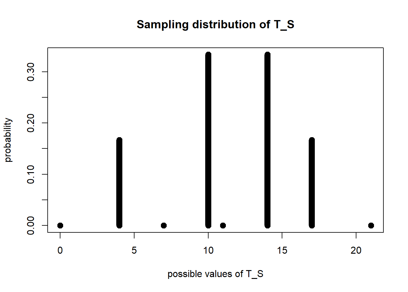

From the plot, we can see that

\[ \P(T_S = 4) = 1/6; \hspace{5mm} \P(T_S = 10) = 1/3; \hspace{5mm} \P(T_S = 14) = 1/3; \hspace{5mm} \P(T_S = 17) = 1/6. \] and the probability that \(T_S\) has other values outside of \(4, 10, 14, 17\) is 0.

2.2.3 Probabilistic Mean

The (probabilistic) mean of a numerical-valued random variable is defined as \[ \E[Z] = \sum_{\text{possible values }z \text{ of }Z} z \times \P(Z = z) \]

Example 2.7 Continue with Example 2.6, the mean of random variable \(Z_1\) is \[ \E[Z_1] = 1 \times \P(Z_1 = 1) + 0 \times \P(Z_1 = 0) = 1 \times 1/2 + 0 \times 1/2 = 1/2. \]

Note here that for a binary random variable \(Z\) having only two possible outcomes \(1\) or \(0\), we always have \[\begin{equation} \E[Z] = 1 \times \P(Z = 1) + 0 \times \P(Z = 0) = \P(Z = 1). \tag{2.5} \end{equation}\]

Example 2.8 Continue with Example 2.6, we have \[\begin{align*} \E[Z_2] = \P(Z_2 = 1) & = \P(S = \{2\}) + \P(S = \{1,2\}) + \P(S = \{2,3\}) + \P(S = \{1,2,3\}) \\ & = 1/3 + 1/3 + 1/6 + 0 = 5/6. \end{align*}\] and \[ \E[Z_3] = \P(Z_3 = 1) = 0 + 0 + 1/6 + 0 = 1/6. \]

2.3 Unbiased Estimator

2.3.1 Bias

Since sample statistics are random, which means it can obtain different values at different repetition of the sampling selection, we need to use the concepts of bias and variance in Section 1.3 to evaluate estimators.

We will first look at bias. Mathematically, bias is defined as \[ \text{Bias}(\hat{\theta}) = \E[\hat{\theta}] - \theta \] If \(\text{Bias}(\hat{\theta}) = 0\), we say \(\hat{\theta}\) is unbiased for \(\theta\). Otherwise, we say that \(\hat{\theta}\) is biased for \(\theta\).

Example 2.9 Continue with Example 2.6, the mean of the sample total \(T_S\) is \[ \E[T_S] = 4 \times 1/6 + 10 \times 1/3 + 14 \times 1/3 + 17 \times 1/6 = 11.5 \] However, we want to estimate the population total, \(t_U = 21\). So the bias of \(T_S\) for \(t_U\) is \[ \E[T_S] - t_U = 11.5 - 21 = -9.5. \]

2.3.2 Bias of Sample Total

To calculate the bias formula of the sample total \(T_S\), we need to calculate its mean. In doing so, we use the following property:

Proposition 2.1 (Linearity of Means) For random variables \(Z_1\), \(Z_2\), and constants (fixed numbers) \(a\) and \(b\), we have \[ \E[aZ_1 + bZ_2] = a\E[Z_1] + b\E[Z_2]. \] In general, if we have \(N\) random variables \(Z_1, ..., Z_N\) and \(N\) constants \(a_1, ..., a_N\), we have \[ \E\left[\sum_{i=1}^N a_iZ_i\right] = \sum_{i=1}^N a_i\E\big[Z_i\big]. \]

Basically, the linearity property of the means says that expectation (i.e., mean) of a linear combination of random variables equals the linear combination of the expectations (i.e., means) of the corresponding random variables.

Applying Property 2.1 to the sample total, we have \[ \E\big[T_S\big] = \E\left[\sum_{i=1}^N Z_iy_i\right] = \sum_{i=1}^N\E\big[Z_i\big]y_i \] where the first equation is from the definition in Equation (2.3), the second equation is from the linearity property of the mean and the design-based framework, which assumes that \(y_i\), \(i=1, ..., N\) are fixed (constants).

So, the bias of the sample total \(T_S\) when estimating the population \(t_U\) is \[ \E\big[T_S\big] - t_U = \sum_{i=1}^N\E\big[Z_i\big]y_i - \sum_{i=1}^Ny_i = \sum_{i=1}^N\Big\{\big(\E[Z_i] - 1\big)y_i\Big\} \] which is often non-zero, meaning that \(T_S\) is often biased for \(t_U\).

Furthermore, note that \(Z_i\), \(i = 1, ..., N\) are binary random variables which can only take one of two values, either 1 or 0, so from Equation (2.5), we have \[ \E\big[Z_i\big] = \P(Z_i = 1) \le 1 \] Now, if \(y_i \ge 0\) for all \(i = 1, ..., N\), for example, when \(Y\) is the monthly rent payment, then \[ \E\big[T_S\big] - t_U = \sum_{i=1}^N\Big\{\big(\E[Z_i] - 1\big)y_i\Big\} = \sum_{i=1}^N\Big\{\big[\P(Z_i = 1) - 1\big]y_i\Big\} \le 0 \] that is, \(T_S\) tends to underestimate \(t_U\) if \(y_i \ge 0\) for all \(i = 1, ..., N\). This is what we have seen in Example 2.9.

The only case where \(T_S\) is unbiased for \(t_U\) is when \(\Pr(Z_i = 1)\) for all \(i = 1, ..., N\). This means that all units \(i\) in the population are included in our sample with certainty, implying that we are taking a census!

2.3.3 Horvitz-Thompson Estimator

From the previous section, we notice that the sample total \(T_S\) is unbiased for the population total \(t_U\) only if we are taking a census. However, as discussed in Section 1.2.2, a census is usually impossible due to constraints in time, cost and other administrative issues. Thus, we cannot use the sample total to estimate the population total and we have to modify the sample total so that it become unbiased!

For this, in 1952, the Horvitz-Thompson estimator is proposed: \[\begin{equation} \hat{T}_{HT} = \sum_{i \in S}\frac{y_i}{\P(Z_i = 1)} = \sum_{i=1}^N \frac{Z_iy_i}{\P(Z_i = 1)}. \tag{2.6} \end{equation}\]

Now, this estimator is unbiased: \[ \E\big[\hat{T}_{HT}\big] = \E\left[\sum_{i=1}^N \frac{Z_iy_i}{\P(Z_i = 1)}\right] = \sum_{i=1}^N\E[Z_i] \frac{y_i}{\P(Z_i = 1)} = \sum_{i=1}^N y_i = t_U \] since \(\E[Z_i] = \Pr(Z_i = 1)\), \(i = 1, ..., N\) by Equation (2.5).

The Horvitz-Thompson estimator is an important mathematical discovery and is the basis for many methods in not only survey sampling but also missing data, causal inference, domain adaptation, etc.

Example 2.6 Continue with Example 2.5. Suppose that \(Y_1 = 4\), \(Y_2 = 10\), \(Y_3 = 7\). The population total is \[ t_U = \sum_{i=1}^3 Y_i = Y_1 + Y_2 + Y_3 = 4 + 10 + 7 = 21. \] From Examples 2.7 and 2.8, we also know that \[ \P(Z_1 = 1) = 1/2; \hspace{5mm} \P(Z_2 = 1) = 5/6; \hspace{5mm} \P(Z_3 = 1) = 1/6 \]

so we can calculate

\(S\)	\(Z_1\)	\(Z_2\)	\(Z_3\)	\(\P(S=s)\)	\(T_S\)	\(\hat{T}_{HT}\)
\(\{\emptyset\}\)	\(0\)	\(0\)	\(0\)	\(0\)	\(0\)	\(0\)
\(\{1\}\)	\(1\)	\(0\)	\(0\)	\(1/6\)	\(4\)	\(4/(1/2) = 8\)
\(\{2\}\)	\(0\)	\(1\)	\(0\)	\(1/3\)	\(10\)	\(10/(5/6) = 12\)
\(\{3\}\)	\(0\)	\(0\)	\(1\)	\(0\)	\(7\)	\(7/(1/6) = 42\)
\(\{1,2\}\)	\(1\)	\(1\)	\(0\)	\(1/3\)	\(14\)	\(8+12= 20\)
\(\{1,3\}\)	\(1\)	\(0\)	\(1\)	\(0\)	\(11\)	\(8+42=50\)
\(\{2,3\}\)	\(0\)	\(1\)	\(1\)	\(1/6\)	\(17\)	\(12+42 = 54\)
\(\{1,2,3\}\)	\(1\)	\(1\)	\(1\)	\(0\)	\(21\)	\(8+12+42 = 62\)

The mean of the Horvitz-Thompson estimator is \[ \E\big[\hat{T}_{HT}\big] = 8 \times \frac{1}{6} + 12 \times \frac{1}{3} + 20 \times \frac{1}{3} + 54 \times \frac{1}{6} = 21 = t_U. \]

So we can see that although the Horvitz-Thompson estimator \(\hat{T}_{HT}\) also results in different values at different sample index set, but on average, it is unbiased for \(t_U\). This is like throwing darts, although the dart may land at different places, but the locations of the landings still surround the bullseye. On the other hand, the sample total \(T_S\) is biased (except for special cases). This is similar to throwing darts but the locations of the landings do not surround the bullseye. Check Figure 2.1 for a visual illustration.

Figure 2.1: Visual illustration of biases of different estimators

Based on the unbiased estimator \(\hat{T}_{HT}\) of the population total, the population mean can also be estimated unbiasedly using the estimator \[\begin{equation} \hat{\bar{Y}}_{HT} = \frac{1}{N}\hat{T}_{HT} = \frac{1}{N}\sum_{i=1}^N\frac{Z_iy_i}{\P(Z_i = 1)} \tag{2.7} \end{equation}\]

Exercise 2.1

1. Prove that \(\hat{\bar{Y}}_{HT}\) is unbiased for the population mean \(\bar{y}_U\).

2. Continue with Example 2.6, calculate \(\hat{\bar{Y}}_{HT}\) for each possible value \(s\) of \(S\). Then calculate \(\E\big[\hat{\bar{Y}}_{HT}\big]\).

2.3.4 Sampling Weights

An important element of the Horvitz-Thompson estimator in Equation (2.6) is the probability \(\P(Z_i = 1)\) for \(i = 1, ..., n\). We will use this probability a lot, so it will be convenient to give it a shorter notation.

• Denote \(\pi_i = \P(Z_i = 1)\) and call this the selection probability of unit \(i\).

• Denote \(w_i = 1/\pi_i\) and call this the sampling weight of unit \(i\).

Now we can write the Horvitz-Thompson estimator as

\[ \hat{T}_{HT} = \sum_{i \in S}\frac{y_i}{\pi_i} = \sum_{i\in S}w_iy_i \]

So, to estimate the population total, each response \(y_i\) of unit \(i\) is weighted by \(w_i\), that is, unit \(i\) needs to represent \(w_i\) units in the population.

The Horvitz-Thompson estimator for the mean is then \[ \hat{\bar{Y}}_{HT} = \frac{1}{N}\hat{T}_{HT} = \frac{1}{N}\sum_{i \in S}\frac{y_i}{\pi_i} = \frac{1}{N}\sum_{i\in S}w_iy_i \]

2.4 Probability Sampling

In Section 2.1.5, we discuss that \(Z\) determines how the sample is obtained and is called the sampling design. In survey sampling, if we can design the sampling process, we can specify and know the probabilities \(\pi_i\), \(i=1, ..., N\). As a result, we can use the Horvitz-Thompson estimator to obtain unbiased estimates!

• We call sampling designs in which we know the sampling probabilities \(\pi_i\) for all units \(i\) in the population probability sampling.

• Non-probability sampling happens when we do not know the sampling probabilities for some (or all) of \(\pi_i\). Examples include self-selection sampling, convenience sampling, and judgement sampling of Section 1.4.1.

Note also that, the Horvitz-Thompson will not work if \(\pi_i = 0\) for some \(i \in U\) because we cannot divide by 0 when we calculate the expectation for \(\hat{T}_{HT}\)!

• In that case, we cannot use the Horvitz-Thompson estimator to correct for bias and need other (often stronger) assumptions.

• Note that \(\pi_i = 0\) for some \(i \in U\) means that there are some units in the population that we cannot reach at all. This implies we have undercoverage (refer to Section 1.4.1).

2.5 Poisson Sampling

2.5.1 The Design

The easiest way to design a sampling scheme is to independently assign a probability \(\frac{n^*}{N}\) of selection for each unit \(i\) in the population. To do so, we

1. Determine a number \(0 < n^* \le N\).

2. For each unit \(i\), independently³ toss a biased coin with \(\frac{n^*}{N}\) chance of resulting in heads.

3. If the result is head, then we select unit \(i\) in our sample. If not, we leave unit \(i\) out of our sample⁴.

This design is called Poisson sampling⁵ in survey sampling context.

In practice, we do not have a biased coin. But we can still do Poisson sampling using a computational software which has a random number generator:

1. Determine a number \(0 < n^* \le N\).

2. For each unit \(i\), independently generate a random variable between \([0,1]\), call this number \(R\).

3. If \(R \le \frac{n^*}{N}\), then we select unit \(i\) in our sample. Otherwise, we leave unit \(i\) out of our sample.

2.5.2 The Estimator

Under Poisson sampling, we know that \(\pi_i = \frac{n^*}{N}\), so we can use this to plug in the Horvitz-Thompson estimator formula in Equation (2.6) and get the estimator for population total: \[ \hat{T}_{HT} = \sum_{i \in S}\frac{y_i}{\pi_i} = \sum_{i \in S}\frac{y_i}{n^*/N} = \frac{N}{n^*}\sum_{i\in S}y_i \]

and the estimator for population mean: \[ \hat{\bar{Y}}_{HT} = \frac{1}{N}\hat{T}_{HT} = \frac{1}{n^*}\sum_{i\in S}y_i \]

Example 2.10 Suppose we design a Poisson sampling with \(n^* = 2\) for a population of 3 units \(\{U = 1, 2, 3\}\). Suppose \(Y_1 = 4\), \(Y_2 = 10\) and \(Y_3 = 7\). Then using the above formulas for \(\hat{T}_{HT}\) and \(\hat{\bar{Y}}_{HT}\):

\(S\)	\(\hat{T}_{HT}\)	\(\hat{\bar{Y}}_{HT}\)
\(\{\emptyset\}\)	\(0\)	\(0\)
\(\{1\}\)	\(4/(2/3) = 6\)	\(6/3 = 4/2 = 2\)
\(\{2\}\)	\(10/(2/3) = 15\)	\(15/3 = 10/2 = 5\)
\(\{3\}\)	\(7/(2/3) = 21/2\)	\((21/2)/3 = 7/2 = 7/2\)
\(\{1,2\}\)	\(6+15 = 21\)	\(21/3 = 14/2 = 7\)
\(\{1,3\}\)	\(6+21/2 = 33/2\)	\((33/2)/3 = 11/2 = 11/2\)
\(\{2,3\}\)	\(15+21/2 = 51/2\)	\((51/2)/3 = 17/2 = 17/2\)
\(\{1,2,3\}\)	\(6+15+21/2 = 63/2\)	\((63/2)/3 = 21/2 = 21/2\)

The difference between between Examples 2.5 and 2.10 is that we did not know the probabilities \(\P(S = s)\) for each possible realized sample index set \(s\). To calculate these probabilities, note that each \(s\) corresponds to a specific value \(\{z_1, ..., z_N\}\) of \(\{Z_1, ..., Z_N\}\). And we will also need to use the independence property of probabilities:

Proposition 2.2 (Independence) If \(Z_1, ..., Z_N\) are independent from one another, \[\begin{align*} \P(Z_1 = z_1, Z_2 = z_2, ..., Z_N = z_n) & = \P(Z_1 = z_1)\times \P(Z_2 = z_2) \times ... \times \P(Z_n = z_n) \\ & = \prod_{i=1}^N \P(Z_1 = z_1). \end{align*}\]

We can apply this to Example 2.10.

Example 2.11 Under Poisson sampling with \(n^* = 2\) and \(N = 3\), we have \[ \P(Z_1 = 1) = \frac{2}{3}, \hspace{5mm} \P(Z_1 = 0) = 1 - \frac{2}{3} = \frac{1}{3} \] Similarly, \[ \P(Z_2 = 1) = \frac{2}{3}, \hspace{5mm} \P(Z_2 = 0) = \frac{1}{3} \] and \[ \P(Z_3 = 1) = \frac{2}{3}, \hspace{5mm} \P(Z_3 = 0) = 1 - \frac{2}{3} = \frac{1}{3} \] Therefore, we can calculate:

\(S\)	\(Z_1\)	\(Z_2\)	\(Z_3\)	\(\P(S = s)\)
\(\{\emptyset\}\)	\(0\)	\(0\)	\(0\)	\(\frac{1}{3} \times \frac{1}{3} \times \frac{1}{3} = \frac{1}{27}\)
\(\{1\}\)	\(1\)	\(0\)	\(0\)	\(\frac{2}{3} \times \frac{1}{3} \times \frac{1}{3} = \frac{2}{27}\)
\(\{2\}\)	\(0\)	\(1\)	\(0\)	\(\frac{1}{3} \times \frac{2}{3} \times \frac{1}{3} = \frac{2}{27}\)
\(\{3\}\)	\(0\)	\(0\)	\(1\)	\(\frac{1}{3} \times \frac{1}{3} \times \frac{2}{3} = \frac{2}{27}\)
\(\{1,2\}\)	\(1\)	\(1\)	\(0\)	\(\frac{2}{3} \times \frac{2}{3} \times \frac{1}{3} = \frac{4}{27}\)
\(\{1,3\}\)	\(1\)	\(0\)	\(1\)	\(\frac{2}{3} \times \frac{1}{3} \times \frac{2}{3} = \frac{4}{27}\)
\(\{2,3\}\)	\(0\)	\(1\)	\(1\)	\(\frac{1}{3} \times \frac{2}{3} \times \frac{2}{3} = \frac{4}{27}\)
\(\{1,2,3\}\)	\(1\)	\(1\)	\(1\)	\(\frac{2}{3} \times \frac{2}{3} \times \frac{2}{3} = \frac{8}{27}\)

From Examples 2.10 and 2.11, we can see that all possible subsets \(s\) of \(U\) have non-zero probability of realization. That is, using Poisson sampling, all possible sizes, from \(0\) to \(N\), have some chance to occur. Thus, \(n^*\) does not necessarily equal to the actual number of units in the sample (i.e., \(n \ne n^*\)), therefore \[ \hat{\bar{Y}}_{HT} = \frac{1}{n^*}\sum_{i\in S}y_i \ne \frac{1}{n}\sum_{i\in S}y_i. \]

Instead, \(n^*\) is the expected value of the sample size: \[ \E\left[\sum_{i=1}^NZ_i\right] = \sum_{i=1}^N \E[Z_i] = \sum_{i=1}^N \frac{n^*}{N} = N\times \frac{n^*}{N} = n^*. \]

2.6 Simple Random Sampling

2.6.1 Definition

From Example 2.11, we can see that using Poisson sampling, we still have positive probabilities of sampling no one from the population (\(S = \emptyset\)), or having to sample everyone from the population (\(S = U\)), which are not ideal. It would be better if we are able to set a fixed sample size \(n\) based on our budget constraints, for example. Furthermore, the HT estimator \(\hat{\bar{Y}}_{HT}\) does not necessary equal the sample mean \(\bar{Y}_S\), which is not convenient.

This motivates us to use simple random sampling (or simple random sampling without replacement), denoted as SRS a sampling method in which we

• select a predetermined sample size \(n\), then

• assign every possible subset of \(n\) distinct units in the population the same probability of happening.

Example 2.12 Again, consider a population of 3 units, i.e., \(U = \{1,2,3\}\) in which \(Y_1 = 4, Y_2 = 10\) and \(Y_3 = 7\). Now, under simple random sampling, if we decide that our sample size should be \(n = 2\), then we have

\(S\)	\(Z_1\)	\(Z_2\)	\(Z_3\)	\(\P(S = s)\)
\(\{\emptyset\}\)	\(0\)	\(0\)	\(0\)	\(0\)
\(\{1\}\)	\(1\)	\(0\)	\(0\)	\(0\)
\(\{2\}\)	\(0\)	\(1\)	\(0\)	\(0\)
\(\{3\}\)	\(0\)	\(0\)	\(1\)	\(0\)
\(\{1,2\}\)	\(1\)	\(1\)	\(0\)	\(1/3\)
\(\{1,3\}\)	\(1\)	\(0\)	\(1\)	\(1/3\)
\(\{2,3\}\)	\(0\)	\(1\)	\(1\)	\(1/3\)
\(\{1,2,3\}\)	\(1\)	\(1\)	\(1\)	\(0\)

That is, there are three possible subsets \(s \subseteq U\) that contain 2 units, so we assign a probability of \(1/3\) to each of them, and assign \(0\) probability to any other possible subsets.

In this case, we have \[ \pi_1 = P(Z_1 = 1) = P(S = \{1,2\}) + P(S = \{1,3\}) = \frac{1}{3} + \frac{1}{3} = \frac{2}{3} \]

\[ \pi_2 = P(Z_2 = 1) = P(S = \{1,2\}) + P(S = \{2,3\}) = \frac{1}{3} + \frac{1}{3} = \frac{2}{3} \]

\[ \pi_3 = P(Z_3 = 1) = P(S = \{1,3\}) + P(S = \{2,3\}) = \frac{1}{3} + \frac{1}{3} = \frac{2}{3} \]

We can see that, in Example 2.12, \(\pi_i\) are the same for every unit \(i \in U\). This is not a coincidence. In fact, in simple random sampling, the selection probability is

\[\begin{equation} \pi_i = \frac{n}{N}, \hspace{5mm} \text{for all } i = 1, 2, ..., N \tag{2.8} \end{equation}\]

where \(n\) is our pre-specified sample size. As a result, the weights \(w_i = 1/\pi_i\) are also the same for all units \(i = 1, ..., N\). Therefore, simple random sampling is also self-weighting.

We can prove that \(\pi_i = n/N\) for any \(i = 1, ..., N\) and arbitrary \(N\) and \(n \le N\).

Proof. First, we notice that there are \(\left( \begin{array}{c} N \\ n \end{array} \right)\) possible subsets of \(n\) distinct units from a population of \(N\) units. This is because we are choosing \(n\) units without replacement from a set of \(N\) units⁶.

Under simple random sampling, we assign equal probabilities to these subsets, so we have \[ P(S = s) = \begin{cases} 1/\left( \begin{array}{c} N \\ n \end{array} \right) & \text{if } s \text{ has } n \text{ units} \\ 0 & \text{otherwise} \end{cases} \]

There are \(\left( \begin{array}{c} N-1 \\ n-1 \end{array} \right)\) possible subsets of \(n\) units that contain unit \(i\). This is because, to create a subset of size \(n\) that contains unit \(i\), we first choose unit \(i\) and put it into our subset. We are then left with \(N-1\) units from the population to choose from, and \(n-1\) empty places in our subset. So the number of ways to choose units for the remaining \(n-1\) places is \(\left( \begin{array}{c} N-1 \\ n-1 \end{array} \right)\). This is also the number of possible subsets of \(n\) distinct units that contain unit \(i\).

In summary, we have \(\left( \begin{array}{c} N \\ n \end{array} \right)\) possible subsets of \(n\) distinct units, each having \(1/\left( \begin{array}{c} N \\ n \end{array} \right)\) chance of happening. Among those subsets, there are \(\left( \begin{array}{c} N-1 \\ n-1 \end{array} \right)\) subsets that contain unit \(i\). Therefore, \[ P(Z_i = 1) = \left( \begin{array}{c} N-1 \\ n-1 \end{array} \right) \times \frac{1}{\left( \begin{array}{c} N \\ n \end{array} \right)} = \frac{n}{N} \]

This applies to any unit \(i\) in the population. So \(\pi_i = n/N\) for all \(i = 1, ..., N\).

2.6.2 The Estimator

Using the results for \(\pi_i\), we can derive the HT estimators for the population mean and population total under simple random sampling: \[ \hat{T}_{HT} = \sum_{i \in S}\frac{y_i}{\pi_i} = \sum_{i \in S}\frac{y_i}{n/N} = \frac{N}{n}\sum_{i\in S}y_i \]

\[ \hat{\bar{Y}}_{HT} = \frac{1}{N}\hat{T}_{HT} = \frac{1}{n}\sum_{i\in S}y_i = \bar{Y}_S \]

So, using simple random sampling, the Horvitz-Thompson estimator for the population mean is the sample mean itself! This is more intuitive and convenient, compared to Poisson sampling!

2.6.3 The Design

There are multiple ways to obtain a simple random sample, say, of sample size \(n\).

The first method is called systematic sampling, which proceeds as follows:

• shuffle the population index set \(U\),

• calculate \(k = \lceil N/n \rceil\), called the ceiling of \(N/n\), which is the smallest integer that is greater or equal to \(N/n\),

• Find a random integer \(R\) between 1 and \(k\)

• Choose units \(R, R+k, R+2k, ..., R+(n-1)k\) into our sample. That is, from the starting point of \(R\), the sampled units will be equally spaced by \(k\) from each other in the shuffled index set.

Example 2.13 Suppose we are interested in obtain an SRS sample of \(n=4\) units from a population of \(N=30\) units.

• First, we shuffle the index set \(U = \{1, 2, ..., 30\}\), and obtain, for example,

  \[\begin{equation} 4,16,13,17,24,26,30,22,6,1,18,27,12,23,14,\\ 25,29,5,10,15,21,11,9,20,7,28,3,8,19,2 \end{equation}\]

• Since \(N/n = 30/4 = 7.5\), the smallest integer that is greater or equal to \(7.5\) is 8, so \(k = 8\).

• We then find a random integer \(R\) between \(1\) and \(k\). Suppose we randomize and get \(R = 5\).

• From the shuffled index set, we first choose the \(R = 5\)th index, then the \(R+k = 13\)th index, the \(R+2k = 21\) index, and finally the \(R+(n-1)k = 5 + (4-1)8 = 29\)th index, which is \[\begin{equation} 4,16,13,17,\color{red}{24},26,30,22,6,1,18,27,\color{red}{12},23,14,\\ 25,29,5,10,15,\color{red}{21},11,9,20,7,28,3,8,\color{red}{19},2 \end{equation}\]

The second method, which is more computer friendly, is to

• generate \(n\) random numbers in \([0,1]\)

• Multiply each number by \(N\)

• Round the result up to the next integer

• If there are duplicates, re-generate a new random number!

Basically, what this does is to divide the range \([0,1]\) into \(N\) equally spaced intervals. We then randomize a number to see which interval contains that number. If the number falls into the \(i\)th interval, then we select that unit into our sample. If two random numbers both fall into the \(i\)th interval, we can select unit \(i\) into our sample, and generate another random number, which may fall into another interval that we did not add into our sample.

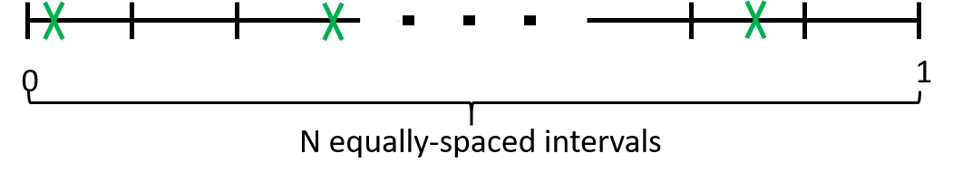
Figure 2.2: Visual illustration of interval-based SRS technique

The third method, which is very convenient in R, is to use the function sample()

sample(1:N, size = n, replace = FALSE) #where N and n are numbers from your survey design 

For example, in Example 2.13, instead of systematic sampling, we can use R

sample(1:30, size = 4, replace = FALSE)

## [1] 29 18 24 28

2.7 Variance

2.7.1 Definition

So far, we have discussed about biases and how we can use the Horvitz-Thompson-estimator to obtain unbiased estimators of the population mean and population total.

Looking at Figure1.2, another aspect of estimators that we need to consider is variance. Variance tells us how each run of an experiment is different from the overall average. Mathematically, it is defined as \[ Var(Z) = \E[(Z - \E[Z])^2], \]

for any random variable \(Z\).

Besides, we also have the definition of the covariance between two random variables \(Z_1, Z_2\):

\[ Cov(Z_1, Z_2) = \E[(Z_1 - \E[Z_1])(Z_2 - \E[Z_2])]. \]

Therefore, \[ Var(Z_1) = Cov(Z_1, Z_1). \]

We can prove that for any random variables \(Z_1, Z_2\): \[\begin{equation} Cov(Z_1, Z_2) = \E[Z_1Z_2] - \E[Z_1]\E[Z_2]. \tag{2.9} \end{equation}\] .

Proof. \[\begin{align*} Cov(Z_1, Z_2) & = \E[(Z_1 - \E[Z_1])(Z_2 - \E[Z_2])] \\ & = \E[(Z_1Z_2 - Z_1\E[Z_2] - \E[Z_1]Z_2 + \E[Z_1]\E[Z_2])] \\ & = \E[Z_1Z_2] - \E[Z_1]\E[Z_2] - \E[Z_1]\E[Z_2] + \E[Z_1]\E[Z_2] \\ & = \E[Z_1Z_2] - \E[Z_1]\E[Z_2]. \end{align*}\]

Therefore \(Var(Z_1) = Cov(Z_1, Z_1) = \E[Z_1^2] - (\E[Z_1])^2\) for any random variable \(Z_1\).

2.7.2 Variance of Horvitz-Thompson Estimators

First, we will start with the Horvitz-Thompson (HT) estimator \(\hat{T}_{HT}\) for the population total.

To derive this variance, we use the variance formula for a linear combination of random variables: \[\begin{equation} Var\left(\sum_{i=1}^Na_iZ_i\right) = \sum_{i=1}^N a_i^2 Var(Z_i) + 2\sum_{i \ne j}a_ia_j Cov(Z_i,Z_j). \tag{2.10} \end{equation}\]

Proof. For two random variables \(Z_1\) and \(Z_2\) and constants \(a_1\), \(a_2\): \[\begin{align*} & Var(a_1Z_1 + a_2Z_2) \\ & = \E\Big[\big\{(a_1Z_1 +a_2Z_2) - \E[a_1Z_1 + a_2Z_2]\big\}^2\Big] \\ & = \E\Big[\big\{(a_1Z_1 - \E[a_1Z_1]) + (a_2Z_2 - \E[a_2Z_2])\big\}^2\Big] \\ & = \E\Big[\big\{(a_1Z_1 - \E[a_1Z_1])^2 + 2(a_1Z_1 - \E[a_1Z_1])(a_2Z_2 - \E[a_2Z_2]) + (a_2Z_2 - \E[a_2Z_2])^2\big\}\Big] \\ & = \E\Big[(a_1Z_1 - \E[a_1Z_1])^2\Big] + 2\E\Big[(a_1Z_1 - \E[a_1Z_1])(a_2Z_2 - \E[a_2Z_2])] + \E\Big[(a_2Z_2 - \E[a_2Z_2])^2\Big] \\ & = a_1^2Var(Z_1) + 2a_1a_2Cov(Z_1,Z_2) + a_2^2Var(Z_2) \end{align*}\] We can then use mathematical induction to prove the case for a linear combination of \(N\) random variables.

Here, \(\sum_{i \ne j} \equiv \sum_{i=1}^N\sum_{j=i+1}^N\), meaning we are summing over all pairs \(i, j\) so that \(i \ne j\).

Now, we apply Equations (2.10) and (2.9) to get

\[\begin{align*} Var(\hat{T}_{HT}) & = Var\left(\sum_{i=1}^N \frac{Z_iy_i}{\pi_i}\right) \\ & = \sum_{i=1}^N\frac{y_i^2}{\pi_i^2}Var(Z_i) + 2\sum_{i\ne j}\frac{y_iy_j}{\pi_i\pi_j}Cov(Z_i, Z_j) \\ & = \sum_{i=1}^N\frac{y_i^2}{\pi_i^2}\pi_i(1-\pi_i) + 2\sum_{i\ne j}\frac{y_iy_j}{\pi_i\pi_j}(\E[Z_iZ_j] - \pi_i\pi_j) \tag{2.11} \end{align*}\]

where the last equation is because \(Z_i\) is a binary random variable, thus \(Z_i = Z_i^2\) and \(\E[Z_i] = \P(Z_i = 1) = \pi_i\), thus \[ Var(Z_i) = \E[Z_i^2] - (\E[Z_i])^2 = \E[Z_i] - (\E[Z_i])^2 = \pi_i - \pi_i^2 = \pi_i(1-\pi_i) \] and \[ Cov(Z_i, Z_j) = \E[Z_iZ_j] - \E[Z_i]\E[Z_j] = \E[Z_iZ_j] - \pi_i\pi_j. \]

And the variance of \(\hat{\bar{Y}}_{HT}\) is \[\begin{equation} Var(\hat{\bar{Y}}_{HT}) = Var\left(\frac{1}{N}\hat{T}_{HT}\right) = \frac{1}{N^2}Var(\hat{T}_{HT}) \tag{2.12} \end{equation}\]

2.7.3 Variance under Simple Random Sampling

In the case of simple random sampling of Section 2.6, we have \(\pi_i = n/N\) and \[ \E[Z_iZ_j] = \P(Z_iZ_j = 1) = \P(Z_i = 1, Z_j = 1) = \left( \begin{array}{c} N-2 \\ n-2 \end{array} \right) \times \frac{1}{\left( \begin{array}{c} N \\ n \end{array} \right)} = \frac{n(n-1)}{N(N-1)} \] since \(Z_1\) and \(Z_2\) are binary random variables so \(Z_1Z_2\) are also binary random variables. Also, \(Z_i = 1\) and \(Z_j = 1\) happens at the same time if both units \(i\) and \(j\) are included in our sample. This is the same as fixing units \(i\) and \(j\) in our sample and having \(N-2\) units left to choose from to fill \(n-2\) remaining positions in our sample.

Plugging the above formulas for \(\pi_i\) and \(\E[Z_iZ_j]\) under SRS to the variance formula of the Horvitz-Thompson estimator in Equation (2.11), we have

\[\begin{equation} Var(\hat{T}_{HT}) = N^2\left(1-\frac{n}{N}\right)\frac{s_U^2}{n}. \tag{2.13} \end{equation}\]

Proof. \[\begin{align*} Var(\hat{T}_{HT}) & = \sum_{i=1}^N\frac{y_i^2}{\pi_i^2}\pi_i(1-\pi_i) + 2\sum_{i\ne j}\frac{y_iy_j}{\pi_i\pi_j}(\E[Z_iZ_j] - \pi_i\pi_j) \\ & = \sum_{i=1}^N\frac{y_i^2}{n^2/N^2}\frac{n}{N}\left(1-\frac{n}{N}\right) + 2\sum_{i\ne j}\frac{y_iy_j}{n^2/N^2}\left(\frac{n(n-1)}{N(N-1)} - \frac{n^2}{N^2}\right) \\ & = \frac{N-n}{n}\sum_{i=1}^Ny_i^2 + 2\frac{-(N-n)}{n(N-1)}\sum_{i\ne j}y_iy_j \\ & = \frac{(N-n)}{n(N-1)}\left\{(N-1)\sum_{i=1}^Ny_i^2 - 2\sum_{i\ne j}y_iy_j\right\} \\ & = \frac{(N-n)}{n(N-1)}\left\{N\sum_{i=1}^Ny_i^2 - \left(\sum_{i=1}^Ny_i^2 + 2\sum_{i\ne j}y_iy_j\right)\right\} \\ & = \frac{(N-n)}{n(N-1)}\left\{N\sum_{i=1}^Ny_i^2 - \left(\sum_{i=1}^Ny_i\right)^2\right\} \\ & = \frac{N(N-n)}{n(N-1)}\left\{\sum_{i=1}^Ny_i^2 - N\left(\frac{1}{N}\sum_{i=1}^Ny_i\right)^2\right\} \\ & = \frac{N(N-n)}{n(N-1)}\left\{\sum_{i=1}^Ny_i^2 - N\bar{y}_U^2\right\} \\ & = \frac{N(N-n)}{n(N-1)}\left\{\sum_{i=1}^Ny_i^2 - 2N\bar{y}_U^2 + N\bar{y}_U^2\right\} \\ & = \frac{N(N-n)}{n(N-1)}\left\{\sum_{i=1}^Ny_i^2 - 2\bar{y}_U\sum_{i=1}^Ny_i + \sum_{i=1}^N\bar{y}_U^2\right\} \\ & = \frac{N(N-n)}{n(N-1)}\left\{\sum_{i=1}^N(y_i^2 - 2y_i\bar{y}_U + \bar{y}_U^2)\right\} \\ & = \frac{N(N-n)}{n(N-1)}\left\{\sum_{i=1}^N(y_i - \bar{y}_U)^2 \right\} \\ & = \frac{N(N-n)}{n}s_U^2 \\ & = N^2\left(1-\frac{n}{N}\right)\frac{s_U^2}{n} \end{align*}\]

where \(s_U^2 = \frac{1}{N-1}\sum_{i=1}^N(y_i - \bar{y}_U)^2\) is the population variance.

Plugging the variance of \(\hat{T}_{HT}\) in Equation (2.14) into the variance formula of the HT estimator \(\hat{\bar{Y}}_{HT}\) for the population mean in Equation (2.12), we have the variance of the HT estimator \(\bar{Y}_S = \hat{\bar{Y}}_{HT}\) for the population mean under SRS: \[\begin{equation} Var(\bar{Y}_S) = \frac{1}{N^2}Var(\hat{T}_{HT}) = \left(1-\frac{n}{N}\right)\frac{s_U^2}{n}. \tag{2.14} \end{equation}\]

In Equations (2.13) and (2.14), the factor \(1-\frac{n}{N}\) is called the finite population correction (or FPC). This is because if \(N\) is not finite, i.e., infinite, and \(n\) is fixed, then this factor will become 1 and the variance of \(\bar{Y}_S\) will be \(s_U^2/n = \sigma^2/n\), which is the variance of \(\bar{Y}_S = 1/n\sum_{i=1}^nY_i\) where we assume that \(Y_1, Y_2, ..., Y_n\) are randomly drawn from a distribution⁷ of variance \(\sigma^2\).

2.7.4 Variance Estimators

In Equations (2.13) and (2.14), the variance formulas involve a population quantity \(s_U^2\), which requires all units in the population. However, we will not know these units unless we sample them and collect data from them!

Therefore, we need to estimate the variance of the HT estimators \(\hat{T}_{HT}\) and \(\hat{\bar{Y}}_{HT}\) from the sample.

In fact, under SRS, the sample variance \(S_S^2 = \frac{1}{n-1}\sum_{i\in S}(y_i - \bar{Y}_S)^2\) is an unbiased estimator of the population variance \(s_U^2\).

Proof. We want to prove \[ \E[S_S^2] = \E\left[\frac{1}{n-1}\sum_{i\in S}(y_i - \bar{Y}_S)^2\right] = \frac{1}{n-1} \E\left[\sum_{i\in S}(y_i - \bar{Y}_S)^2\right] = s_U^2, \] which is equivalent to proving \(\E\left[\sum_{i\in S}(y_i - \bar{Y}_S)^2\right] = s_U^2\). This is because: \[\begin{align*} \E\left[\sum_{i\in S}(y_i - \bar{Y}_S)^2\right] & = \E\Big[\sum_{i\in S}\big(\{y_i - \bar{y}_U\} - \{\bar{Y}_S - \bar{y}_U\}\big)^2\Big] \\ & = \E\Big[\sum_{i\in S}\big(\{y_i - \bar{y}_U\}^2 - 2\{y_i - \bar{y}_U\}\{\bar{Y}_S - \bar{y}_U\} + \{\bar{Y}_S - \bar{y}_U\}^2\big)\Big] \\ & = \E\Big[\sum_{i\in S}\{y_i - \bar{y}_U\}^2 - 2\{\bar{Y}_S - \bar{y}_U\}\sum_{i\in S}\{y_i - \bar{y}_U\} + n\{\bar{Y}_S - \bar{y}_U\}^2\Big] \\ & = \E\Big[\sum_{i\in S}\{y_i - \bar{y}_U\}^2 - 2n\{\bar{Y}_S - \bar{y}_U\}^2 + n\{\bar{Y}_S - \bar{y}_U\}^2\Big] \\ & = \E\Big[\sum_{i\in S}\{y_i - \bar{y}_U\}^2 - n\{\bar{Y}_S - \bar{y}_U\}^2\Big] \\ & = \E\Big[\sum_{i\in S}\{y_i - \bar{y}_U\}^2\Big] - n\Big[\{\bar{Y}_S - \bar{y}_U\}^2\Big] \\ & = \E\Big[\sum_{i=1}^NZ_i\{y_i - \bar{y}_U\}^2\Big] - nVar(\bar{Y}_S) \\ & = \sum_{i=1}^N(\E[Z_i]\{y_i - \bar{y}_U\}^2) - nVar\left(\frac{1}{N}\hat{T}_{HT}\right) \\ & = \frac{n}{N}\sum_{i=1}^N\{y_i - \bar{y}_U\}^2 - \frac{n}{N^2}Var\left(\hat{T}_{HT}\right) \\ & = \frac{n}{N}(N-1)s_U^2 - \frac{n}{N^2}N^2\left(1-\frac{n}{N}\right)\frac{s_U^2}{n} \\ & = (n-1)s_U^2, \end{align*}\] where the 7th equation is because under SRS, \(\bar{Y}_S\) is an unbiased estimator for \(\bar{y}_U\), so \(\bar{y}_U = \E[\bar{Y}_S]\); and the 10th equation is obtained by applying Equation (2.13).

Therefore, under SRS, we can estimate the variance of the HT estimators \(\hat{T}_{HT}\) and \(\hat{\bar{Y}}_{HT}\) by \[\begin{equation} \hat{Var}(\hat{T}_{HT}) = N^2\left(1-\frac{n}{N}\right)\frac{S_S^2}{n}. \tag{2.15} \end{equation}\] and \[\begin{equation} \hat{Var}(\bar{Y}_S) = \frac{1}{N^2}Var(\hat{T}_{HT}) = \left(1-\frac{n}{N}\right)\frac{S_S^2}{n}. \tag{2.16} \end{equation}\]

Exercise 2.2

1. Derive the variance formula for the HT estimators under Poisson sampling, using the fact that if \(Z_i\) and \(Z_j\) are independent, then \(Cov(Z_i, Z_j) = 0\).

2. Suggest an estimator for the variance of the HT estimators under Poisson sampling. Hint: using an HT estimator for the variance itself!

The standard error of an estimator \(\hat{\theta}\) is defined as the square root of the variance, that is \(SE(\hat{\theta}) = \sqrt{Var(\hat{\theta})}\). Therefore, the standard errors of the HT estimators for population total and populaton mean under SRS can be estimated by taking the square root of the formula in Equations (2.15) and (2.16), which gives \[\begin{equation} \hat{SE}(\hat{T}_{HT}) = N\sqrt{1-\frac{n}{N}}\frac{S_S}{\sqrt{n}}. \tag{2.17} \end{equation}\] and \[\begin{equation} \hat{SE}(\bar{Y}_S) = N\sqrt{1-\frac{n}{N}}\frac{S_S}{\sqrt{n}}. \tag{2.18} \end{equation}\] Note here the difference between the standard error \(SE\), which is the square root of the variance of an estimator, and the standard deviation \(S_S\) or \(s_U\), which is the square toot of the observations \(y\) in our sample or population, respectively.

Example 2.14 Take an SRS of 4 units from a population of 10 units and obtain \(y_1 = 2\), \(y_2 = 6\), \(y_3=3\), \(y_4=10\).

The HT estimator for the population mean \(\hat{\bar{Y}}_{HT}\), i.e., the sample mean \(\bar{Y}_S\) (since we are sampling under SES), is \[ \bar{Y}_S = \frac{1}{4}(2+6+3+10) = \frac{21}{4} \] The sample variance is \[ S_S^2 = \frac{1}{4-1}\left\{\left(2-\frac{21}{4}\right)^2 + \left(6-\frac{21}{4}\right)^2 + \left(3-\frac{21}{4}\right)^2 + \left(10-\frac{21}{4}\right)^2\right\} = 12.9167 \] The variance of the sample mean is \[ \hat{Var}(\bar{Y}_S) = \left(1-\frac{4}{10}\right)\frac{12.9167}{4} = 1.9375 \] The standard deviation is \[ \hat{SE}(\bar{Y}_S) = \sqrt{1.9375} = 1.3919 \]

We can also use survey package in R to calculate the HT estimates, which are the realized values of the estimators on a specific sample. Suppose your sample is stored in variable y of a dataset called your_sample.

y <- your_data
your_sample <- data.frame(y = y) 
#here, the left-hand side of y=y is the name of the variable
#the right-hand side of y=y is the vector that contains your data

First, we need to specify the SRS design

library(survey)
design.srs <- svydesign(ids = ~1, 
                        data = your_sample, 
                        fpc = ~rep(N,n))

Then use the following commands to obtain the estimate for population mean

svymean(x = ~y, design = design.srs)

The estimate for population total can be obtained by

svytotal(x = ~y, design = design.srs)

Example 2.15 Continue with Example 2.14, we can use R to obtain our estimates:

library(survey)
y <- c(2,6,3,10)
your_sample <- data.frame(y = y) 
design.srs <- svydesign(ids = ~1, 
                        data = your_sample, 
                        fpc = ~rep(10,4))
svymean(x = ~y, design = design.srs)

##   mean     SE
## y 5.25 1.3919

This gives the same results as our calculation in Example 2.14.

Proportion is a special case of means, where the variable of interest \(Y\) is binary, for example, whether a student has a private washroom at their residence. Let \(p_U\) denote the population proportion and \(\hat{P}_S\) denote the sample proportion. Note that \[ \bar{Y}_S = \hat{P}_S = \frac{1}{n}\sum_{i=1}^ny_i = \frac{\text{# of units } i \text{ so that }y_i=1}{n} \]

Then with some algebra, we can prove that \[\begin{equation} s_U^2 = \frac{N}{N-1}p_U(1-p_U) \tag{2.19} \end{equation}\]

Proof. Since \(y_i\)’s are binary, we have \[\begin{align*} s_U^2 & = \frac{1}{N-1}\sum_{i=1}^N(y_i - p_U)^2 \\ & = \frac{1}{N-1} \left(\sum_{i: y_i = 0}p_U^2 + \sum_{i: y_i = 1}(1-p_U)^2\right) \\ & = \frac{1}{N-1} \left(p_U^2N(1-p_U) + (1-p_U)^2Np_U\right) \\ & = \frac{1}{N-1}Np_U(1-p_U)(p_U + 1-p_U) \\ & = \frac{N}{N-1}p_U(1-p_U) \end{align*}\] where the third equation is because we are summing over all unit \(i\)’s such that \(y_i = 0\), and there are \(N(1-p_U)\) such units in the population. Similarly, we are summing over \(Np_U\) units with \(y_i = 1\).

Similarly, we have \(S_S^2 = \frac{n}{n-1}\hat{P}_S(1-\hat{P}_S)\).

Therefore, the HT estimator for population proportion under SRS is \(\hat{\bar{Y}}_{HT} = \bar{Y}_S = \hat{P}_S\) and the estimated variance is obtained by plugging in the formula for \(S_S^2\) into Equation (2.16): \[\begin{equation} \hat{Var}(\hat{P}_S) = \left(1-\frac{n}{N}\right)\frac{\hat{P}_S(1-\hat{P}_S)}{n-1} \tag{2.20} \end{equation}\]

Example 2.16 Suppose we take an SRS of 30 students from a population of 100 students, and observe in our sample that \(10\%\) of students have private washroom.

Then we can use \(\hat{P}_S = 10\% = 0.1\) to estimate the proportion of students in the population that have private washroom.

The estimated variance of this estimate is \[ \hat{Var}(\hat{P}_S) = \left(1-\frac{30}{100}\right)\frac{0.1\times(1-0.1)}{30-1} = 0.0022 \] and the standard error is \(\sqrt{0.0022} = 0.0469\).

2.8 Confidence Intervals

A \(100(1-\alpha)\%\) confidence interval is defined as an interval \((LB_S, UB_S)\) which satisfies \[\begin{equation} \P(LB_S \le \theta \le UB_S) = 1-\alpha. \tag{2.21} \end{equation}\]

To construct confidence intervals for HT estimators, we use the Central Limit Theorem for HT estimators Berger (1998): \[\begin{equation} \frac{\hat{\theta}_{HT} - \theta}{SE(\hat{\theta}_{HT})} \to \mathcal{N}(0,1). \tag{2.22} \end{equation}\] This is called the asymptotic normality of the HT estimators. The asymptotic here means that if the population size \(N\) goes to infinity, the sample size \(n\) also goes to infinity, and \(N-n\) goes to infinity, then \((\hat{\theta}_{HT} - \theta)/SE(\hat{\theta}_{HT})\) will follows a standard normal distribution. In practice, if \(y\) roughly follows normal distribution, then with \(n \ge 30\) and \(N >> n\), we can apply the central limit theorem (Lohr 2021).

Based on the Central Limit Theorem, we have \[\begin{equation} \P\left(\left|\frac{\hat{\theta}_{HT}-\theta}{SE(\hat{\theta}_{HT})}\right| \le z_{\alpha/2}\right) = 1-\alpha, \tag{2.23} \end{equation}\] where \(z_{\alpha/2}\) is the \(1-\alpha/2\) quantile of the standard normal distribution. This is the same as \[ \P\Big(\hat{\theta}_{HT} - z_{\alpha/2}SE(\hat{\theta}_{HT}) \le \theta \le \hat{\theta}_{HT} + z_{\alpha/2}SE(\hat{\theta}_{HT})\Big) = 1-\alpha. \] Compare this to Equation (2.21), we see that, in our case, \[ LB_S = \hat{\theta}_{HT} - z_{\alpha/2}SE(\hat{\theta}_{HT}) \hspace{5mm} \text{and} \hspace{5mm} UB_S = \hat{\theta}_{HT} + z_{\alpha/2}SE(\hat{\theta}_{HT}) \] and the confidence interval is \[ \hat{\theta}_{HT} \pm z_{\alpha/2}SE(\hat{\theta}_{HT}) = (\hat{\theta}_{HT} - z_{\alpha/2}SE(\hat{\theta}_{HT}), \hat{\theta}_{HT} + z_{\alpha/2}SE(\hat{\theta}_{HT})) \] Usually, we use \(\alpha = 0.05\) to obtain \(95\%\) CI and thus \(z_{\alpha/2} = 1.96\).

We can see that \(LB_S\) and \(UB_S\) are calculated from the sample, which is why I used the subscript \(S\) in the notation. Therefore, if we repeat the sample selection process, we will receive a different confidence interval. Furthermore, if we repeat the sample selection process many times, then \(100(1-\alpha)\%\) of the obtained confidence intervals will contain the true value. See Figure 2.3 for an illustration. In general, we say for short that we are \(100(1 − \alpha)\%\) confident that \(\theta\) lies in the interval.

Figure 2.3: Visual illustration of confidence intervals. The red dotted line represents the true value⁸.

In R, we can obtain the confidence interval by using the code:

est.total <- svytotal(x = ~y, design = design.srs)
confint(est.total)

and

est.mean <- svymean(x = ~y, design = design.srs)
confint(est.mean)

Example 2.17 In Example 2.14, the \(95\%\) confidence interval is \[ \frac{21}{4} \pm 1.96 \times 1.3919 = (2.5219, 7.9781). \] In R, we can write

est.mean <- svymean(x = ~y, design = design.srs)
confint(est.mean)

##      2.5 %   97.5 %
## y 2.521846 7.978154

In Example 2.16, the \(95\%\) confidence interval is \[ 0.1 \pm 1.96 \times 0.0469 = (0.0081, 0.1919). \]

2.9 Sample Size Determination

In Sections 2.6, we see that, in order to perform SRS, we need to specify the sample size \(n\). In practice, sample size determination is useful for us to prepare for resources before we roll out our study and conduct the surveys to collect information/data. Usually, we have limited resources, so we will want a small sample size.

Moreover, from Equation (2.14), as sample size \(n\) increases, the variance of \(\hat{\bar{Y}}_{HT} = \bar{Y}_S\) decreases. So in this case, we want the sample size to be big so that our estimates are more precise.

To reconcile these two objectives, usually sample sizes are determined based on the following statement: we want a sample size \(n\) so that \[\begin{equation} \P\left(\left|\hat{\theta}-\theta\right| \le e\right) = 1-\alpha, \tag{2.24} \end{equation}\] where \(e\) is called the margin of error. This means that instead of surveying the whole population to get the exact population quantities like in a census, we want to survey a small sample while tolerating some errors \(e\) with confidence \(1-\alpha\).

From Equation (2.23), we can see that, in our survey sampling setting with HT estimators, \[\begin{equation} e = z_{\alpha/2}SE(\hat{\theta}), \tag{2.25} \end{equation}\] Since \(SE(\hat{\theta}_{HT})\) is related to \(n\), we can solve Equation (2.25) to obtain the desired sample size \(n\). Note that \(n\) is an integer, if a non-integer number is obtained while solving Equation (2.25), we then round up the number to get the desired sample size (we better sample more).

Now, if our HT estimator of interest is \(\bar{Y}_S\), then \[ e = z_{\alpha/2}\sqrt{1-\frac{n}{N}}\frac{s_U}{\sqrt{n}} \]

Solving the above equation, we obtain \[\begin{equation} n = \frac{z_{\alpha/2}^2s_U^2}{e^2 + \frac{z_{\alpha/2}^2s_U^2}{N}} \tag{2.26} \end{equation}\]

Proof. \[\begin{align*} & e = z_{\alpha/2}\sqrt{1-\frac{n}{N}}\frac{s_U}{\sqrt{n}} \\ & \Leftrightarrow e^2 = z_{\alpha/2}^2\left(1-\frac{n}{N}\right)\frac{s_U^2}{n} \\ & \Leftrightarrow \frac{e^2}{z_{\alpha/2}^2s_U^2} = \frac{1}{n} - \frac{1}{N} \\ & \Leftrightarrow n = \frac{1}{\frac{e^2}{z_{\alpha/2}^2s_U^2} + \frac{1}{N}} \\ & \Leftrightarrow n = \frac{z_{\alpha/2}^2s_U^2}{e^2 + \frac{z_{\alpha/2}^2s_U^2}{N}} \end{align*}\]

Example 2.18 We are conducting an SRS from a population of \(N = 1251\) students to estimate the mean rent. If the population standard deviation is \(\$300\), we can tolerate an error of \(\$100\) with \(95\%\) confidence. Then the sample size we need is

\[ n = \frac{1.96^2\times 300^2}{100^2 + \frac{1.96^2\times 300^2}{1251}} = 33.6446 \] So the sample size we need is 34 students.

In general, we do not know \(s_U^2\) and cannot estimate it before we conduct the survey. We may guess its value based on a pilot study, a previous study in the literature, or from an educated guess from the domain expert.

However, when what we are interested in is the proportion, from algebra, we know that for \(0 \le p_U \le 1\), \(p_U(1-p_U) = \frac{1}{4} - (x-\frac{1}{2})^2 \le \frac{1}{4}\). We can use this to estimate the largest value of \(s_U^2\): \[ s_U^2 = \frac{N}{N-1}p_U(1-p_U) \approx p_U(1-p_U) \le \frac{1}{4}. \] Here, the approximation happens when \(N\) is large. Now, we can use this maximum value of \(s_U^2\) to plug in Equation (2.26) to get a conservative sample size, i.e., a sample size that is possibly larger than needed, but we’re better safe than sorry.

Example 2.19 Suppose we want to estimate the proportion of students who have private washroom. We plan to take an SRS from a population of \(N=1251\) students, and want to use \(95\%\) with margin or error \(0.03\). The sample size we need is \[ n = \frac{1.96^2\times \frac{1}{4}}{0.03^2 + \frac{1.96^2\times \frac{1}{4}}{1251}} = 575.8809 \to 576. \]

In Example 2.18, we see that \(s_U\) has unit of Canadian dollar. In that case, for different study we need to specify a specific value of \(s_U\) depending on the unit of the response variable \(Y\). Instead, we may know the relative ratio between the standard deviation and the mean, for example, from a study about student rent in the US where the data is collected in US dollar. Now, the ratio \(CV = s_U/\bar{y}_U\), which is called the coefficient of variation, can help us! This is because the coefficient of variation does not have a unit, i.e., it is scale-free. Specifically, we can make a statement like this: we want a sample size \(n\) so that \[\begin{equation} \P\left(\left|\frac{\hat{\theta}-\theta}{\theta}\right| \le r\right) = 1-\alpha, \tag{2.27} \end{equation}\] where \(r\) is called the relative precision. In case of wanting to estimate the population mean under SRS, we can determine, in the similar fashion as in Equation (2.26), that \[ n = \frac{z_{\alpha/2}^2(s_U/\bar{y}_U)^2}{r^2 + \frac{z_{\alpha/2}^2(s_U/\bar{y}_U)^2}{N}}, \]

where \(s_U/\bar{y}_U\) is the coefficient of variation!

Example 2.20 Suppose we want to estimate the mean rent payments of students. We plan to take an SRS from a population of \(N=1251\) students, and want to use \(95\%\) with relative precision \(0.3\). The population coefficient of variation is estimated to be \(0.8\). The sample size needed is: \[ n = \frac{1.96^2\times 0.8^2}{0.3^2 + \frac{1.96^2\times 0.8^2}{1251}} = 26.7343 \to 27. \]