3 Stratified Sampling

3.1 What is Stratified Sampling?

3.1.1 Components

Stratified sampling is composed of two steps:

• Stratification: Divide the population into \(H\) subpopulations, called strata,

  • Each subpopulation is called a stratum

  • The variable used to divide population is called the stratification variable.

  • The strata: (i) do not overlap and (ii) constitute the whole population, such that each sampling unit belongs to exactly one stratum⁹.

• Sampling: Draw an independent probability sample from each stratum.

  • Recall from Section 2.4 that a probability sample is when we know the sampling or inclusion probability for each unit in the population.

  • If we draw a non-probability sample in each stratum, that is called quota sampling instead of startified sampling.

  • In this chapter, we consider taking independent Simple Random Sampling (SRS) sample from each stratum. Check Section 2.6 for a refresh on SRS.

Figure 3.1 illustrates stratified sampling, where the population is divided into strata of different colors, and from each of the stratum, some units are selected randomly and added into the sample.

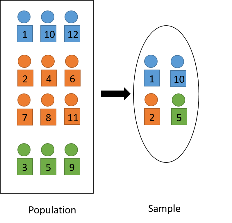
Figure 3.1: Visual illustration of stratified sampling technique.

Example 3.1 In the students’ rent Example 1.1, we can divide the students at USask by their college affiliation such that each student is only affiliated to one college. Stratified sampling is when we independently take an SRS from each of the colleges. Now, college affiliation is the stratification variable.

3.1.2 Why Stratification?

Stratification is usually used because

• It is more convenient to administer the survey and may lower costs

  • Imagine having to get an email list of all students at the university, versus asking each college their student email list.

• Sometimes we want inference for subgroups

  • Instead of only wanting to know the mean rent payment of all students at the university, we may also want to know the mean rent payment of students from each college specifically.

• Improve representativeness of the sample

  • If we take an SRS from the whole university, we may end up with a sample without any student from Arts and Science. However, with stratified sampling, our sample will contain students from all colleges at USask.

• As we will see in later sections, stratified sampling usually gives more precise (i.e., lower variance) estimates for population means and totals.

3.2 Estimation

3.2.1 Population Parameters

Suppose we divide the population \(U\) of \(N\) units into \(H\) strata: \(U_1, U_2, ..., U_H\). Note that, by definition in Section 3.1.1:

• These strata do not overlap, i.e., \(U_h \cap U_l = \emptyset\) for \(1 \le h \ne l \le H\).

• These strata comprise the full population, i.e., \(U = U_1 \cup U_2 \cup ... \cup U_H\).

Suppose the \(h\)th stratum \(U_h\) contains \(N_h\) units, then \(\sum_{h=1}^H N_h = N\).

Let \(y_{h,i}\) denote the response of the \(i\)th unit in the \(h\)th stratum.

We then have the population and subpopulation parameters as follows:

	Stratum (subpopulation) \(h\)	Population
Total	\(\color{red}{t_{U,h} = \sum_{i=1}^{N_h}y_{h,i}}\)	\(\color{red}{t_U = \sum_{h=1}^H t_{U,h}} = \sum_{h=1}^H\sum_{i=1}^{N_h}y_{h,i}\)
Mean	\(\color{red}{\overline{y}_{U,h} = \frac{1}{N_h}t_{U,h}} = \frac{1}{N_h} \sum_{i=1}^{N_h}y_{h,i}\)	\(\color{red}{\overline{y}_U = \frac{1}{N}t_U} = \frac{1}{N}\sum_{h=1}^H\sum_{i=1}^{N_h}y_{h,i}\)
Variance	\(\color{red}{s_{U,h}^2} = \frac{1}{N_h-1}\sum_{i=1}^{N_h}(y_{h,i}-\overline{y}_{U,h})^2\)	\(\color{red}{s_U^2} = \frac{1}{N-1}\sum_{h=1}^H\sum_{i=1}^{N_h}(y_{h,i}-\overline{y}_U)^2\)

Notes: We cannot average the subpopulation means to get the overall population mean, i.e., \(\overline{y}_U \ne \frac{1}{H}\overline{y}_{U,h}\). This is because \(\overline{y}_{U,h}\) is the mean that represents \(N_h\) units in the population. Therefore, we have to use a weighted average instead, with each \(\overline{y}_{U,h}\) weighted by the fraction of number of units in stratum \(h\) out of the whole population, i.e., \(N_h/N\). \[ \overline{y}_U = \frac{1}{N}\sum_{h=1}^H\sum_{i=1}^{N_h}y_{h,i}=\sum_{h=1}^H\frac{N_h}{N}\overline{y}_{U,h} \]

3.2.2 Sample and HT Estimators

As defined in Section 3.1.1, for each \(h\), we take an SRS sample \(S_h\) of \(n_h\) units from stratum \(U_h\). Then our overall sample consists of units from these subsets: \(S = S_1 \cup S_2 \cup ... \cup S_H\) and the overall sample size is \(n = \sum_{h=1}^H n_h\).

Since we take an SRS from each of the stratum, we can use the HT estimators in Section 2.5.2 to estimate the subpopulation means and totals. By aggregating these subpopulation HT estimators, we can get the HT estimators for the population mean and total. The order is:

• First, calculate the HT estimates for the subpopulation means \(\widehat{\overline{Y}}_{HT,h}\). Since subpopulations are sampled using SRS, HT estimates for subpopulation means are the sample means, i.e., \(\widehat{\overline{Y}}_{HT,h} = \overline{Y}_{S,h}\)

• Now, calculate the HT estimates for the subpopulation totals \(\widehat{T}_{HT,h}\), which equals the estimates of the subpopulation means times the number of units in the subpopulation: \(\widehat{T}_{HT,h} = N_h\widehat{\overline{Y}}_{HT,h}\).

• Then, calculate the HT estimate for the overall population total \(\widehat{T}_{HT}\) by summing the HT estimates of the subpopulation totals: \(\widehat{T}_{HT} = \sum_{h=1}^H \widehat{T}_{HT,h}\).

• Finally, calculate the HT estimate for the overall population mean \(\widehat{\overline{Y}}_{HT}\) by dividing the HT estimate for the overall population total by the number of units in the population: \(\widehat{\overline{Y}}_{HT} = \frac{1}{N}\widehat{T}_{HT}\).

The process is summarized in the table below:

	HT estimators for stratum \(h\)	HT estimators for whole population
Mean	\(\color{red}{\widehat{\overline{Y}}_{HT,h} = \overline{Y}_{S,h}} = \frac{1}{n_h} \sum_{i \in S_h}y_{h,i}\)	\(\color{red}{\widehat{\overline{Y}}_{HT} = \frac{1}{N}\widehat{T}_{HT}} = \frac{1}{N}\sum_{h=1}^H\sum_{i=1}^{N_h}y_{h,i}\)
Total	\(\color{red}{\widehat{T}_{HT,h} = N_h\widehat{\overline{Y}}_{HT,h}} = \frac{N_h}{n_h} \sum_{i \in S_h}y_{h,i}\)	\(\color{red}{\widehat{T}_{HT} = \sum_{h=1}^H \widehat{T}_{HT,h}} = \sum_{h=1}^H N_h\widehat{\overline{Y}}_{HT,h}\)

Notes: Here, the HT estimator for the overall population mean is not equal to the overall sample mean, i.e., \(\widehat{\overline{Y}}_{HT} \ne \overline{Y}_S\). This is the result for SRS only. Here, we are dealing with stratified sampling, not SRS.

3.2.3 Variances

In stratified sampling, SRS samples are taken independently from each stratum. Therefore, we can derive that \[\begin{equation} Var_{strt}\left(\widehat{T}_{HT}\right) = \sum_{h=1}^H Var_{SRS}(\widehat{T}_{HT,h}) = \sum_{h=1}^H N_h^2\left(1-\frac{n_h}{N_h}\right)\frac{s^2_{U,h}}{n_h}. \tag{3.1} \end{equation}\]

Proof. Recall in Section 2.7.2, we derived the variance of a general HT estimator as \[ Var(\widehat{T}_{HT}) = \sum_{i=1}^N\frac{y_i^2}{\pi_i^2}Var(Z_i) + 2\sum_{i\ne j}\frac{y_iy_j}{\pi_i\pi_j}Cov(Z_i, Z_j) \] We can apply this to stratified sampling and derive

\[\begin{align*} Var_{strt}(\widehat{T}_{HT}) & = \sum_{i=1}^N\frac{y_i^2}{\pi_i^2}Var(Z_i) + 2\sum_{i\ne j}\frac{y_iy_j}{\pi_i\pi_j}Cov(Z_i, Z_j) \\ & = \sum_{h=1}^H\sum_{i=1}^{N_h}\frac{y_{h,i}^2}{\pi_{h,i}^2}Var(Z_{h,i}) + 2\sum_{h=1}^H\sum_{i\ne j, i \in U_h, j \in U_h}\frac{y_{h,i}y_{h,j}}{\pi_{h,i}\pi_{h,j}}Cov(Z_{h,i}, Z_{h,j}) \\ & \qquad + 2\sum_{h=1}^H\sum_{i \in U_h, j \in U_l, h\ne l}\frac{y_{h,i}y_{l,j}}{\pi_{h,i}\pi_{l,j}}Cov(Z_{h,i}, Z_{l,j}) \\ & = \sum_{h=1}^H\left(\sum_{i=1}^{N_h}\frac{y_{h,i}^2}{\pi_{h,i}^2}Var(Z_{h,i}) + 2\sum_{i\ne j, i \in U_h, j \in U_h}\frac{y_{h,i}y_{h,j}}{\pi_{h,i}\pi_{h,j}}Cov(Z_{h,i}, Z_{h,j})\right) \\ & = \sum_{h=1}^H Var_{SRS}(\widehat{T}_{HT,h}) \end{align*}\]

In the second equation, I first divide the population into subpopulations \(U_h\), \(h=1, 2, ..., H\). I then divide all pairs \(i,j\) into two categories: (i) units \(i\) and \(j\) are in the same stratum or (ii) they are in different strata. In the third equation, since SRS are taken independently from each stratum, if units \(i\) and \(j\) are from different strata, then \(Cov(Z_{h,i}, Z_{l,j}) = 0\). Finally, the last equation happens because SRS samples are taken from each stratum.

Similarly, since \(\widehat{\overline{Y}}_{HT} = \frac{1}{N}\widehat{T}_{HT}\), we have \(Var\left(\widehat{\overline{Y}}_{HT}\right) = \frac{1}{N^2}Var\left(\widehat{T}_{HT}\right)\), and therefore:

\[\begin{equation} Var_{strt}\left(\widehat{\overline{Y}}_{HT}\right) = \sum_{h=1}^H Var_{SRS}(\widehat{\overline{Y}}_{HT,h}) = \sum_{h=1}^H \left(1-\frac{n_h}{N_h}\right)\frac{s^2_{U,h}}{n_h}. \tag{3.2} \end{equation}\]

3.2.4 Variance Estimators

From Equations (3.1) and (3.2) and the fact that each subpopulation are sampled using SRS, we can use the SRS variance estimators for each subpopulation and sum them together to get the variance estimators for the population, that is: \[\begin{equation} \widehat{Var}_{strt}\left(\widehat{T}_{HT}\right) = \sum_{h=1}^H \widehat{Var}_{SRS}(\widehat{T}_{HT,h}) = \sum_{h=1}^H N_h^2\left(1-\frac{n_h}{N_h}\right)\frac{S^2_{S,h}}{n_h}, \tag{3.3} \end{equation}\] and \[\begin{equation} \widehat{Var}_{strt}\left(\widehat{\overline{Y}}_{HT}\right) = \sum_{h=1}^H \widehat{Var}_{SRS}(\widehat{\overline{Y}}_{HT,h}) = \sum_{h=1}^H \left(1-\frac{n_h}{N_h}\right)\frac{S^2_{S,h}}{n_h}. \tag{3.4} \end{equation}\] In other words, in Equations (3.1) and (3.2), we replace the subpopulation variances \(s^2_{U,h}\) by the sub-sample variances \(S^2_{S,h}\).

Example 3.2 Suppose we conducted stratified sampling and collected the following information:

Stratum	\(N_h\)	\(n_h\)	\(\overline{Y}_{S,h}\)	\(S_{S,h}^2\)	\(\widehat{T}_{HT,h}\)	\(\widehat{Var}_{SRS}(\widehat{T}_{HT,h})\)
\(A\)	\(100\)	\(20\)	\(7\)	\(2\)	\(100 \times 7 = 700\)	\(100^2\times \left(1-\frac{20}{100}\right)\times \frac{2}{20} = 800\)
\(B\)	\(200\)	\(40\)	\(4\)	\(4\)	\(200 \times 4 = 800\)	\(200^2\times \left(1-\frac{40}{200}\right)\times \frac{4}{40} = 3200\)
\(C\)	\(300\)	\(50\)	\(6\)	\(3\)	\(300 \times 6 = 1800\)	\(300^2\times \left(1-\frac{50}{300}\right)\times \frac{3}{50} = 4500\)

To estimate the overall population total, we have

• \(\widehat{T}_{HT} = \widehat{T}_{HT, A} + \widehat{T}_{HT, B} + \widehat{T}_{HT, C} = 700 + 800 + 1800 = 3300\)

• \(\widehat{Var}(\widehat{T}_{HT}) = \widehat{Var}(\widehat{T}_{HT, A}) + \widehat{Var}(\widehat{T}_{HT, B}) + \widehat{Var}(\widehat{T}_{HT, C}) = 8500\)

• 95% CI: \(3300 \pm 1.96 \times \sqrt{8500} = (3119.297, 3480.703)\)

To estimate the overall population mean, we have

• \(\widehat{\overline{Y}}_{HT} = \frac{1}{N}\widehat{T}_{HT} = \frac{3300}{600} = 5.5\).

• \(\widehat{Var}(\widehat{\overline{Y}}_{HT}) = \frac{1}{N^2}\widehat{Var}(\widehat{T}_{HT}) = \frac{8500}{600^2} = 0.0236\)

• 95% CI: \(5.5 \pm 1.96 \times \sqrt{0.0236} = (5.1989, 5.8011)\)

3.3 Design

3.3.1 Approaches

In Chapter 2, we considered two sampling schemes, Poisson sampling and SRS. To designa Poisson sampling, we only need to specify only one design feature, which is the expected sample size \(n^*\). Similarly, for SRS, we only need to specify the sample size \(n\).

In stratified sampling, we need to consider two design features, that is, we need to:

• define the stratification variable, and

• determine the sample size \(n_h\) in each stratum \(h = 1,2, ..., H\).

There are two approaches to the design of stratified sampling.

First approach: Suppose we want precise estimates \(\widehat{T}_{HT,h}\) or \(\widehat{\overline{Y}}_{HT,h}\) for each stratum \(h\). In this case,

• the stratification variable is already well-defined from our research interest

• we only need to determine a tolerable margin of error \(e_h\) for each stratum \(h\), then proceed to separately calculate sample size \(n_h\) for each stratum \(h\) just like in SRS (see Section 2.9).

Second approach:

• For a fixed general sample size \(n\), determine an allocation rule for \(n_h\) such that \[ n = n_1 + n_2 + ... + n_H. \]

• Based on the allocation rule, we

  • Derive the formula of \(Var_{strt}(\widehat{T}_{HT,h})\) or \(Var_{strt}(\widehat{\overline{Y}}_{HT,h})\) so that the formula is related to \(n\).

  • Solve for \(n\) based on the formula and the tolerable margin of error \(e\).

  • Determine \(n_h\) for each \(h = 1, 2, ..., H\) from the allocation rule.

We will explore more about the second approach in the following sections.

3.3.2 Proportional Allocation

3.3.2.1 Definition and Properties

Proportional allocation is when we sample proportional to the size of the stratum, that is

\[\begin{equation} n_h \propto N_h. \tag{3.5} \end{equation}\]

This means that there is a constant \(k\), which is not dependent on \(h\), such that \(n_h = kN_h\) for all \(h = 1, 2, ..., H\). However, we also know that \(\sum_{h=1}^Hn_h = n\).

This implies \[\begin{equation} \frac{n}{N} = \frac{n_1}{N_1} = \frac{n_2}{N_2} = ... = \frac{n_H}{N_H}. \tag{3.6} \end{equation}\]

Proof. We have \[\begin{align*} n & = \sum_{h=1}^Hn_h \\ & = \sum_{h=1}^H kN_h \\ & = k \sum_{h=1}^H N_h \\ & = k N \end{align*}\] Therefore, \(k = \frac{n}{N}\) and thus \(n_h = \frac{n}{N}N_h\) and \(\frac{n_h}{N_h} = \frac{n}{N}\) for all \(h = 1, 2, ..., H\).

With proportional allocation, the sample is a miniature version of the population, and thus, the sample is representative of the population in terms of the stratification variable.

An illustration of proportional allocation is given in Figure 3.2, where we take a sample of \(\frac{1}{3}\) the size of the population. The sample comprises of sub-samples that are \(\frac{1}{3}\) the size of each stratum. The resulting sample is representative of the population in terms of color: one half of the sample is orange, one fourth is blue and the other one fourth is green.

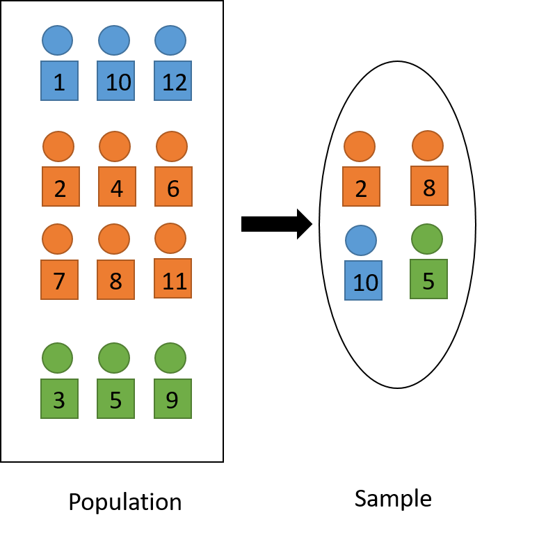
Figure 3.2: Visual illustration of proportional allocation.

Example 3.3 Consider sampling from a population of \(N_1=2400\) men and \(N_2=1600\) women. If we take a \(10\%\) stratified sample with proportional allocation, our sample will have \(n_1 = N_1 \times 10\% = 240\) men and \(n_2 = N_2 \times 10\% = 160\) women. The sample now has the same proportions of men and women as the population.

Another property of stratified sampling with proportional allocation is that it is self-weighting: the probability that the \(i\)th unit from stratum \(h\) is included in our sample is \(\pi_{h,i} = \frac{n_h}{N_h} = \frac{n}{N}\), since we do SRS within each stratum. Therefore, the weight for the \(i\)th unit from stratum \(h\) is \(w_{h,i} = \frac{1}{\pi_{h,i}} = \frac{N}{n}\), which is the same across all units and strata. We also have that \[ \widehat{T}_{HT} = \sum_{h=1}^H \widehat{T}_{HT,h} = \sum_{h=1}^H\sum_{i\in S_h}\frac{N_h}{n_h}y_{h,i} = \sum_{h=1}^H\sum_{i\in S_h}\frac{N}{n}y_{h,i} \] In other words, each unit in the sample \(S = S_1 \cup ...\cup S_h\) represents the same number of units, i. \(\frac{N}{n}\), in the population.

Example 3.4 Continuing with Example 3.3, each unit in our sample will represent \(\frac{1}{10\%}= 10\) people in the population.

3.3.2.2 Variances

Plugging \(\frac{n_h}{N_h} = \frac{n}{N}\) into Equation (3.1), we get \[\begin{equation} Var_{strt,prop}\left(\widehat{T}_{HT}\right) = \frac{N}{n}\left(1-\frac{n}{N}\right)\sum_{h=1}^HN_hs_{U,h}^2. \tag{3.7} \end{equation}\]

Proof. We have \[\begin{align*} Var_{strt,prop}(\widehat{T}_{HT}) & = \sum_{h=1}^H Var_{SRS}(\widehat{T}_{HT,h}) \\ & = \sum_{h=1}^H N_h^2\left(1-\frac{n_h}{N_h}\right)\frac{s_{U,h}^2}{n_h} \\ & = \sum_{h=1}^H N_h \frac{N_h}{n_h}\left(1-\frac{n_h}{N_h}\right)s_{U,h}^2 \\ & = \frac{N}{n}\left(1-\frac{n}{N}\right)\sum_{h=1}^HN_hs_{U,h}^2. \end{align*}\]

Similarly, \[\begin{equation} Var_{strt,prop}\left(\widehat{\overline{Y}}_{HT}\right) = \frac{1}{nN}\left(1-\frac{n}{N}\right)\sum_{h=1}^HN_hs_{U,h}^2. \tag{3.8} \end{equation}\]

3.3.2.3 Comparing to SRS

In this section, we explore whether stratification is worthwhile, or whether we have better use SRS, in terms of estimating the population total (or mean). Note that in both cases, we are using the Horvitz-Thompson estimator, so we are unbiased. We only need to compare the variance then.

Recall from Equation (2.13) that the variance of the Horvitz-Thompson estimator for the population total under SRS is

\[\begin{equation} Var_{SRS}\left(\widehat{T}_{HT}\right) = N^2\left(1-\frac{n}{N}\right)\frac{s_U^2}{n} = \frac{N}{n}\left(1-\frac{n}{N}\right)Ns_U^2 \tag{3.9} \end{equation}\]

On the other hand, from Equation (3.7), the variance of the Horvitz-Thompson estimator for the population total under stratified sampling with proportional allocation is:

\[\begin{equation} Var_{strt,prop}\left(\widehat{T}_{HT}\right) = \frac{N}{n}\left(1-\frac{n}{N}\right)\sum_{h=1}^HN_hs_{U,h}^2. \tag{3.10} \end{equation}\]

Therefore, to compare \(Var_{SRS}\left(\widehat{T}_{HT}\right)\) and \(Var_{strt,prop}\left(\widehat{T}_{HT}\right)\), we need to compare \(Ns_U^2\) and \(\sum_{h=1}^HN_hs_{U,h}^2\). To make this comparison easier, we define

Sum of Squares	Notation	Formula	Meaning
Between	\(SSB\)	\(\sum_{h=1}^HN_h(\overline{y}_{U,h} - \overline{y}_U)^2\)	Between-strata variation
Within	\(SSW\)	\(\sum_{h=1}^H\sum_{i=1}^{N_h}(y_{h,i}-\overline{y}_{U,h})^2\)	Within-stratum variation
Total	\(SST\)	\(\sum_{h=1}^H\sum_{i=1}^{N_h}(y_{h,i}-\overline{y}_U)^2\)	Total variation

The within-stratum variation measures the differences of units to its respective means, the between-strata variation measures the differences of the stratum means to the overall means, and the total variation measures the differences of units to the overall means.

Example 3.5 For example, the within-stratum variation sums over the differences such as of an Arts and Science student’s monthly rent payment to the Arts and Science mean, the between-stratum variation sums over the differences such as of the Arts and Science mean to the USask mean, and the total variation sums over the differences such as of a student to the USask mean.

We can prove that \(SST = SSW + SSB\).

Proof. We have \[\begin{align*} SST & = \sum_{h=1}^H\sum_{i=1}^{N_h}(y_{h,i}-\overline{y}_U)^2 \\ & = \sum_{h=1}^H\sum_{i=1}^{N_h}\left([y_{h,i}- \overline{y}_{U,h}] - [\overline{y}_U - \overline{y}_{U,h}] \right)^2 \\ & = \sum_{h=1}^H\sum_{i=1}^{N_h}(y_{h,i}- \overline{y}_{U,h})^2 + \sum_{h=1}^H\sum_{i=1}^{N_h}(\overline{y}_U - \overline{y}_{U,h})^2 - 2\sum_{h=1}^H\sum_{i=1}^{N_h}(y_{h,i}- \overline{y}_{U,h})(\overline{y}_U - \overline{y}_{U,h}) \\ & = \sum_{h=1}^H\sum_{i=1}^{N_h}(y_{h,i}- \overline{y}_{U,h})^2 + \sum_{h=1}^HN_h(\overline{y}_U - \overline{y}_{U,h})^2 - 2\sum_{h=1}^H(\overline{y}_U - \overline{y}_{U,h})\sum_{i=1}^{N_h}(y_{h,i}- \overline{y}_{U,h}) \\ & = \sum_{h=1}^H\sum_{i=1}^{N_h}(y_{h,i}- \overline{y}_{U,h})^2 + \sum_{h=1}^HN_h(\overline{y}_{U,h} - \overline{y}_U)^2 - 2\sum_{h=1}^H(\overline{y}_U - \overline{y}_{U,h})\left[\left(\sum_{i=1}^{N_h}y_{h,i}\right) - \left(N_h\overline{y}_{U,h}\right) \right] \\ & = SSW + SSB - 2\sum_{h=1}^H(\overline{y}_U - \overline{y}_{U,h})\left[t_{U,h} - t_{U,h}\right) \right] \\ & = SSW + SSB - 0 \\ & = SSW + SSB \end{align*}\]

Using the definitions of \(SST, SSB\) and \(SSW\), we have

\[ Ns_U^2 = \frac{N}{N-1}\sum_{h=1}^H\sum_{i=1}^{N_h}(y_{h,i}-\overline{y}_U)^2 = \frac{N}{N-1}SST = \frac{N}{N-1}(SSW + SSB) \] and \[\begin{align*} \sum_{h=1}^H N_hs_{U,h}^2 & = \sum_{h=1}^H\frac{N_h}{N_h-1}\sum_{i=1}^{N_h}(y_{h,i}-\overline{y}_{U,h})^2 = \sum_{h=1}^H\left(1+\frac{1}{N_h-1}\right)\sum_{i=1}^{N_h}(y_{h,i}-\overline{y}_{U,h})^2 \\ & = SSW + \sum_{h=1}^H s_{U,h}^2 \end{align*}\]

Plugging these into the formula of (3.9) and (3.10) we have \[\begin{equation} Var_{SRS}\left(\widehat{T}_{HT}\right) - Var_{strt,prop}\left(\widehat{T}_{HT}\right) = \frac{N}{n}\left(1-\frac{n}{N}\right) \frac{N}{N-1} \left[ SSB - \sum_{h=1}^H \left(1-\frac{N_h}{N}\right) s_{U,h}^2 \right]. \tag{3.11} \end{equation}\]

Proof. \[\begin{align*} Var_{SRS}\left(\widehat{T}_{HT}\right) - Var_{strt,prop}\left(\widehat{T}_{HT}\right) & = \frac{N}{n}\left(1-\frac{n}{N}\right) \left[ \frac{N}{N-1}(SSW + SSB) - \left(SSW + \sum_{h=1}^H s_{U,h}^2 \right) \right] \\ & = \frac{N}{n}\left(1-\frac{n}{N}\right) \left[ \frac{N}{N-1}SSB + \frac{1}{N-1}SSW - \sum_{h=1}^H s_{U,h}^2 \right] \\ & = \frac{N}{n}\left(1-\frac{n}{N}\right) \left[ \frac{N}{N-1}SSB + \frac{1}{N-1}SSW - \sum_{h=1}^H s_{U,h}^2 \right] \\ & = \frac{N}{n}\left(1-\frac{n}{N}\right) \left[ \frac{N}{N-1}SSB + \sum_{h=1}^H \frac{N_h-1}{N-1} s_{U,h}^2 - \sum_{h=1}^H s_{U,h}^2 \right] \\ & = \frac{N}{n}\left(1-\frac{n}{N}\right) \left[ \frac{N}{N-1}SSB - \sum_{h=1}^H \frac{N-N_h}{N-1} s_{U,h}^2 \right] \\ & = \frac{N}{n}\left(1-\frac{n}{N}\right) \frac{N}{N-1} \left[ SSB - \sum_{h=1}^H \left(1-\frac{N_h}{N}\right) s_{U,h}^2 \right] \\ \end{align*}\]

This is greater or equal to 0, that is, the variance from SRS is larger than the variance from stratification under proportional allocation, if \[ SSB \ge \sum_{h=1}^H \left(1-\frac{N_h}{N}\right) s_{U,h}^2 \] This happens if \(SSB\) is large and \(s^2_{U,h}\) are small, for \(h = 1, 2, ..., H\). Therefore, to reduce variance using stratification, we should choose a stratification variable so that

• it is closely related with (i.e., predictive) of the variable of interest \(Y\)

• so that stratum means \(\overline{y}_{U,h}\) are as different as possible, and

• unit responses \(y_{h,i}\) are similar within a stratum

On another note, we also can prove that if \(N_h\) and \(N\) are large, then variance from stratified sampling under proportional allocation is always smalller than variance from SRS. In other words, we always gain efficiency (i.e., lower variance) with stratification and proporational allocation when strata sizes are large.

Proof. When \(N_h\) and \(N\) are large, \[ Ns^2_U = \frac{N}{N-1}SST \approx SST = SSB + SSW \] and \[ \sum_{h=1}^H N_hs_{U,h}^2 = \sum_{h=1}^H\frac{N_h}{N_h-1}\sum_{i=1}^{N_h}(y_{h,i}-\overline{y}_{U,h})^2 \approx \sum_{h=1}^H\sum_{i=1}^{N_h}(y_{h,i}-\overline{y}_{U,h})^2 = SSW \] Since \(SSB\) is a sum of squares, it is always positive. Therefore, \(Ns^2_U \ge \sum_{h=1}^H N_hs_{U,h}^2\), and thus \(Var_{SRS}\left(\widehat{T}_{HT}\right) \ge Var_{strt,prop}\left(\widehat{T}_{HT}\right)\) and we always gain efficiency.

Example 3.6 Since the number of students in each college is large, we are gaining efficiency when stratifying by college affiliation and do proportional allocation.

In contrast, if the stratum sizes are small, stratum means \(\overline{y}_{U,h}\) are similar, and within-stratum variation is large, we will lose efficiency by stratification. In that case, we prefer to use SRS.

Example 3.7 Suppose we have two strata:

Stratum	\(y_{h,i}\)	\(\overline{y}_{U,h}\)	\(s_{U,h}^2\)
\(1\)	\(4,9,5\)	\(\frac{1}{3}(4+9+5) = 6\)	\(\frac{1}{3-1}\left[(4-6)^2+(9-6)^2+(5-6)^2\right] = 7\)
\(2\)	\(6,7,8\)	\(\frac{1}{3}(6+7+8) = 7\)	\(\frac{1}{3-1}\left[(6-7)^2+(7-7)^2+(8-7)^2\right] = 1\)

We can see that, in this case, \(\overline{y}_{U,1}\) is very similar to \(\overline{y}_{U,2}\). At the same time, \(s_{U,1}^2\) is large. We expect that stratification is hurting us. In fact, we have

\[ SSB = \sum_{h=1}^H N_h(\overline{y}_{U,h} - \overline{y}_U)^2 = 3\times (6-6.5)^2 + 3\times (7-6.5)^2 = 1.5, \]

which is smaller than

\[ \sum_{h=1}^H\left(1-\frac{N_h}{N}\right)s_{U,h}^2 = \left(1-\frac{3}{6}\right)\times 7 + \left(1-\frac{3}{6}\right)\times 1 = 4. \]

Exercise 3.1 In Example 3.7, can you re-define two strata, each with 3 units, so that stratification with proportional allocation is better than SRS?

3.3.3 Optimal Allocation

3.3.3.1 Definition

As discussed in Section 2.9, in survey sampling, we want to balance two contraries: (i) we want to have a large sample size so that the variance of our estimators are the smallest, on the other hand (ii) we only have limited time and resources to collect the survey information. Optimal allocation is a method in stratified sampling that explicitly minimizes the variance of the HT estimators within a fixed cost constraints.

To formalize this mathematically, let

• \(c_0\) be the known overhead cost of the survey

  • This can be the costs to start the survey such as administrative cost to apply for funding for the survey, to travel to or contact the survey hubs, etc.

• \(c_h\) be the known cost to sample one unit from stratum \(h\)

  • This can be the cost to print the survey questionnaire, labor costs to interview individuals, etc.

Suppose we have a fixed budget \(C\), then our unknown (or to-be-determined) sub-sample sizes \(n_1, n_2, ..., n_H\) must satisfy \[ C = c_0 + \sum_{h=1}^H c_hn_h, \] while at the same time minimize¹⁰ \[ Var_{strt}(\widehat{T}_{HT}) = \sum_{h=1}^H Var_{SRS}(\widehat{T}_{HT,h}) = \sum_{h=1}^H N_h^2 \left(1-\frac{n_h}{N_h}\right)\frac{s_{U,h}^2}{n_h}. \]

This is a constrained optimization problem where the objective is to minimize the variance subject to the budget constraint. We can prove that the solution \(n_1, ..., n_H\) for this problem satisfy \[\begin{equation} n_h \propto \frac{N_hs_{U,h}}{\sqrt{c_h}} \tag{3.12} \end{equation}\]

Proof. We can solve this constraint optimization by using Lagrange multiplier. In particular, we form the function \[ f(n_1, n_2, ..., n_H, \lambda) = \sum_{h=1}^H N_h^2 \left(1-\frac{n_h}{N_h}\right)\frac{s_{U,h}^2}{n_h} - \lambda \left(C - c_0 - \sum_{h=1}^H c_hn_h\right) \] Take partial derivatives of \(f\) with respect to \(n_h\) and set them to 0 we get \[ \frac{\partial f}{\partial n_h} = -\frac{N_h^2s_{U,h}^2}{n_h^2} + \lambda c_h = 0 \] This implies \[ n_h = \frac{1}{\sqrt{\lambda}} \frac{N_hs_{U,h}}{\sqrt{c_n}} \propto \frac{N_hs_{U,h}}{\sqrt{c_h}}. \]

From Equation (3.12), we can see that in optimal allocation, we will sample more in a stratum \(h\) if

• \(c_h\) is small, which means it is cheaper to sample there, and/or

• \(N_h\) is large, which means the stratum has a lot of units and we need to sample more there to lower our variance, and/or

• \(s_{U,h}\) is large, which means the responses vary a lot in that stratum and we need to sample more there to lower our variance.

Using the same argument as in Equation (3.6), we have \[ n_h = \left(\frac{\frac{N_hs_{U,h}}{\sqrt{c_h}}}{\sum_{l=1}^H \frac{N_ls_{U,l}}{\sqrt{c_l}}}\right)n. \]

3.3.3.2 Neyman Allocation

A special case of optimal allocation is Neyman allocation. When the costs to sample one unit from each stratum are the same, that is, \(c_1 = c_2 = ... = c_H\), then optimal allocation becomes Neyman allocation, where

\[\begin{equation} n_h \propto N_hs_{U,h} \tag{3.13} \end{equation}\]

Under stratified sampling with Neyman allocation, the variance of the HT estimator for the population mean is
\[\begin{equation} Var_{strt,Ney}(\widehat{T}_{HT}) = \frac{1}{n}\left(\sum_{h=1}^H N_hs_{U,h}\right)^2 - \sum_{h=1}^H N_hs_{U,h}^2. \tag{3.14} \end{equation}\]

Proof. Neyman allocation implies \[ n_h = \left(\frac{N_hs_{U,h}}{\sum_{l=1}^H N_ls_{U,l}}\right)n \] Pluggin this into the variance formula for the HT estimator of the population total under stratified sampling, we have \[\begin{align*} Var_{strt}(\widehat{T}_{HT}) & = \sum_{h=1}^H Var_{SRS}(\widehat{T}_{HT,h}) = \sum_{h=1}^H N_h^2 \left(1-\frac{n_h}{N_h}\right)\frac{s_{U,h}^2}{n_h} \\ & = \sum_{h=1}^H N_h^2\frac{s_{U,h}^2}{n_h} - \sum_{h=1}^H N_hs_{U,h}^2 \\ & = \sum_{h=1}^H N_h^2 \frac{s_{U,h}^2 \sum_{l=1}^H N_ls_{U,l}}{N_hs_{U,h} n} - \sum_{h=1}^H N_hs_{U,h}^2 \\ & = \frac{1}{n}\sum_{h=1}^H N_hs_{U,h} \sum_{l=1}^H N_ls_{U,l} - \sum_{h=1}^H N_hs_{U,h}^2 \\ & = \frac{1}{n}\left(\sum_{h=1}^H N_hs_{U,h}\right)^2 - \sum_{h=1}^H N_hs_{U,h}^2. \\ \end{align*}\]

We can prove that, for same sample size \(n\), Neyman allocation is more efficient that proportional allocation, that is
\[\begin{equation} Var_{strt,Ney}(\widehat{T}_{HT}) \le Var_{strt,prop}(\widehat{T}_{HT}). \tag{3.15} \end{equation}\]

Proof. Consider \[\begin{align*} & Var_{strt,prop}(\widehat{T}_{HT}) - Var_{strt,Ney}(\widehat{T}_{HT}) \\ & \qquad = \frac{N}{n}\left(1-\frac{n}{N}\right)\sum_{h=1}^HN_hs_{U,h}^2 - \left(\frac{1}{n}\left(\sum_{h=1}^H N_hs_{U,h}\right)^2 - \sum_{h=1}^H N_hs_{U,h}^2\right) \\ & \qquad = \frac{N}{n}\sum_{h=1}^HN_hs_{U,h}^2 - \sum_{h=1}^HN_hs_{U,h}^2 - \frac{1}{n}\left(\sum_{h=1}^H N_hs_{U,h}\right)^2 + \sum_{h=1}^H N_hs_{U,h}^2 \\ & \qquad = \frac{N}{n}\sum_{h=1}^HN_hs_{U,h}^2 - \frac{1}{n}\left(\sum_{h=1}^H N_hs_{U,h}\right)^2 \\ & \qquad = \frac{N^2}{n}\left[\sum_{h=1}^H\frac{N_h}{N}s_{U,h}^2 - \left(\sum_{h=1}^H \frac{N_h}{N}s_{U,h}\right)^2\right] \\ & \qquad = \frac{N^2}{n}\sum_{h=1}^H\frac{N_h}{N}(s_{U,h} - \bar{s})^2 \ge 0, \end{align*}\] where \(\bar{s} = \sum_{h=1}^N\frac{N_h}{N}s_{U,h}\).

3.3.3.3 Comparing to Proportional Allocation

Recall that

• Proportional allocation: \(n_h \propto N_h\)

• Optimal allocation: \(n_h \propto \frac{N_hs_{U,h}}{\sqrt{c}_h}\)

So optimal allocation is the same as proportional allocation when \(s_{U,1} = s_{U,2} = ... = s_{U,H}\) and \(c_{U,1} = c_{U,2} = ... = c_{U,H}\).

Note that although it is better than proportional allocation since it is the optimizer, optimal allocation only works for one variable of interest because the allocation depends on \(s_{U,h}\), which in turn depends on \(y_{h,i}\). Often, in survey sampling, we have more than one variable of interest. For example, not only we are interested in students’ rent payment, but we may also be interested in other expenses as well. If \(s_{U,h}\) and \(c_{U,h}\) are almost the similar among clusters, the gain in doing optimal allocation is small and we better use proportional allocation.

Example 3.8 Suppose we want to sample \(n = 36\) students for a survey about test scores. To design this year’s survey, we consider two strata of sizes 1200 and 800, respectively, and we take the means and standard deviations from last year’s survey and get

Stratum	\(N_h\)	\(\overline{y}_{U,h}\)	\(s_{U,h}\)	\(N_h s_{U,h}\)	\(N_h s_{U,h}^2\)
\(1\)	\(1,200\)	\(60\)	\(15\)	\(18,000\)	\(270,000\)
\(2\)	\(800\)	\(80\)	\(10\)	\(8,000\)	\(80,000\)
Total	\(2,000\)			\(26,000\)	\(350,000\)

If we use stratified sampling, proportional allocation:

• Since \(n_h = \frac{n}{N}N_h\), \(n_1 = \frac{36}{2000}\times 1200 = 21.6 \approx 22\) and \(n_2 = \frac{36}{2000} \times 800 = 14.4 \approx 14\).

• \(Var_{strt, prop}(\widehat{T}_{HT}) = \frac{N}{n}\left(1-\frac{n}{N}\right)\sum_{h=1}^HN_hs_{U,h}^2 = \frac{2000}{36}\left(1 - \frac{36}{2000}\right)350,000=19,094,444\).

• \(Var_{strt, prop}(\widehat{\overline{Y}}_{HT}) = \frac{1}{N^2}Var_{strt, prop}(\widehat{T}_{HT}) = 4.7736\)

If we use stratified sampling, Neyman allocation:

• Since \(n_h = \left(\frac{N_hs_{U,h}}{\sum_{l=1}^H N_ls_{U,l}}\right)n\), \(n_1 = \frac{18,000}{26,000}\times 36 = 24.9231 \approx 25\) and \(n_2 = \frac{8,000}{26,000} \times 36 = 11.0769 \approx 11\).

• \(Var_{strt, Ney}(\widehat{T}_{HT}) = \frac{1}{n}\left(\sum_{h=1}^H N_hs_{U,h}\right)^2 - \sum_{h=1}^H N_hs_{U,h}^2\) \(= \frac{1}{36}\times 26,000^2 - 350,000 = 18,427,778\)

• \(Var_{strt, Ney}(\widehat{\overline{Y}}_{HT}) = \frac{1}{N^2}Var_{strt, Ney}(\widehat{T}_{HT}) = 4.6069\)

If we use SRS,

• \(Var_{SRS}(\widehat{T}_{HT}) = N^2\left(1-\frac{n}{N}\right)\frac{s_U^2}{n} = N^2\left(1-\frac{n}{N}\right)\frac{(SSB+SSW)}{n(N-1)}\)

• \(SSB = \sum_{h=1}^H N_h(\overline{y}_{h,U} - \overline{y}_U)^2 = 1,200 \times (60-68)^2 + 800 \times (80-68)^2 = 192,000\).

• \(SSW = \sum_{h=1}^H (N_h - 1)s_h^2 = 350,000 - 15^2 - 10^2 = 349,675\)

• \(Var_{SRS}(\widehat{T}_{HT}) = 2000^2\times \left(1 - \frac{36}{2000}\right)\frac{192,000 + 349,675}{36\times 1999} = 29,566,164\).

• \(Var_{SRS}(\widehat{\overline{Y}}_{HT}) = \frac{1}{N^2}Var_{SRS}(\widehat{T}_{HT}) = 7.3915\).

3.3.4 Design Effect

The design effect of a complex survey is defined as \[ DE = \frac{Var_{complex}(\widehat{\overline{Y}})}{Var_{SRS}(\widehat{\overline{Y}})}, \]

in which the variances are calculated based on sample size \(n\). The interpretation of design effect is that we gain/lose \(DE\times 100\%\) of efficiency when using the complex sampling design instead of SRS. Furthermore, we need \(\frac{n}{DE}\) observations under SRS to achieve the same variance as in the complex sampling scheme with \(n\) observations. We call \(n_{eff} = \frac{n}{DE}\) the effective sample size.

Example 3.9 In Example 3.8, the design effect of stratified sampling with proportional allocation is \[ \frac{Var_{strt, prop}(\widehat{\overline{Y}}_{HT})}{Var_{SRS}(\widehat{\overline{Y}}_{HT})} = \frac{4.7736}{7.3915} =0.6458 \] This means that we need \(36/0.65 = 23.4 \approx 55\) observations in SRS to achieve the same variance as in the stratified sample with proportional allocation with \(36\) observations. The effective sample size here is \(55\).

3.3.5 Sample Size Determination

Similar to Section 2.9, for proportional allocation, \[ Var_{strt, prop}(\widehat{\overline{Y}}_{HT}) = \frac{1}{n}\left(1-\frac{n}{N}\right)\sum_{h=1}^H\frac{N_h}{N}s_{U,h}^2 \] so setting the tolerable margin of error \(e = z_{\alpha/2}\sqrt{Var_{strt, prop}(\widehat{\overline{Y}}_{HT})}\), we can calculate the sample size to be \[ n_{prop} = \frac{\sum_{h=1}^H\frac{N_h}{N}s_{U,h}^2}{\frac{e^2}{z_{\alpha/2}^2} + \frac{1}{N}\sum_{h=1}^H\frac{N_h}{N}s_{U,h}^2} \]

For Neyman allocation, since \[ Var_{strt, Ney}(\widehat{\overline{Y}}_{HT}) = \frac{1}{n}\left(\sum_{h=1}^H \frac{N_h}{N}s_{U,h}\right)^2 - \frac{1}{N}\sum_{h=1}^H \frac{N_h}{N}s_{U,h}^2. \] so setting the tolerable margin of error \(e = z_{\alpha/2}\sqrt{Var_{strt, Ney}(\widehat{\overline{Y}}_{HT})}\), we can calculate the sample size to be \[ n_{Ney} = \frac{\left(\sum_{h=1}^H\frac{N_h}{N}s_{U,h}\right)^2}{\frac{e^2}{z_{\alpha/2}^2} + \frac{1}{N}\sum_{h=1}^H\frac{N_h}{N}s_{U,h}^2}. \]