A Introduction to R
A.1 Why R?
When conducting analyses of data sets with hundreds to thousands of observations, calculating by hand is not feasible and you will need a statistical software. R is one of those. R can also be thought of as a high-level programming language. In fact, R is one of the top languages to be used by data analysts and data scientists. There are a lot of analysis packages in R that are currently developed and maintained by researchers around the world to deal with different data problems. And most importantly, R is free. In this book, we will learn how to use R to conduct basic statistical analyses.
A.2 Installing R and RStudio
To install R, go to the following link: https://www.r-project.org/. You can choose the CRAN closest to your location.
To work with R more easily, download RStudio, an interface software for R, from the following link: https://www.rstudio.com/products/rstudio/download/. The free version is good enough for our use.
After downloading, install R and RStudio on your computer following the instruction of the installation .exe file.
A.3 The RStudio Interface
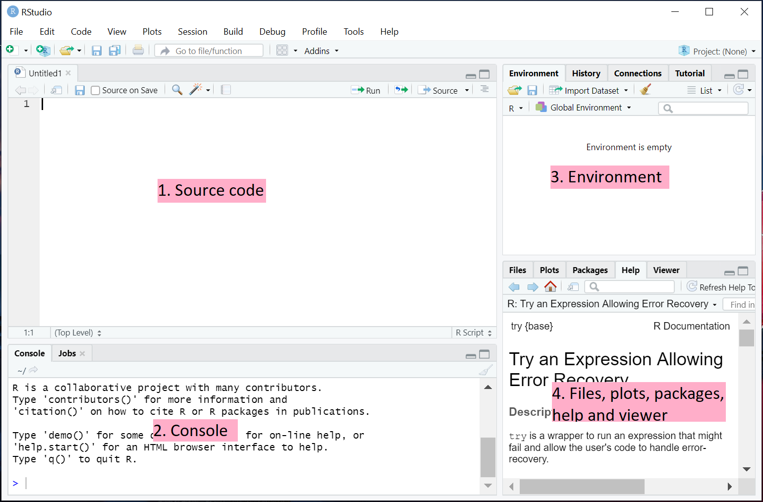
When you open RStudio, the below window will pop up.

Figure A.1: RStduio windows
Notice that there are four panels in the RStudio window.
Source code panel: This is where we write scripts that contains codes to be saved for later use. You can create a new R script by clicking the white button below File and choose R Script.
Console panel: This is where we execute the codes (in our script) interactively and where we see the printed output of the code. We can run our code by
selecting the code in our script file and click run, or
typing or pasting the code in the console, then hit Enter.
The output of our code will appear in the console.
Environment panel:
The Environment tab shows the active datasets or variables that are currently saved in R’s working memory.
The History tab keeps track of every single line of code that has been entered and run through the console.
The Files, Plots, Packages, Help and Viewer panel:
The Plots tab shows the plots (or graphs) that we create using our code.
The Files tab keep track of the files in our working directory.
The Packages tab will show available packages in our local R library.
The Help tab will show documentation about the packages or functions if we ask.
A.4 Helper Codes
A.4.1 Packages
In R, packages contain functions that will become handy when you conduct data analyses. You can view the available CRAN packages in your library or search for a specific package in the Packages tab.
To install packages in R, you can run the code
replacing packagename by the name of the package.
Once a package is installed we need to load them in order to use their functions using the code
Note that a package is only installed once but needs to be loaded every time we want to use its functions.
A.4.2 Getting Help
install.packages() and library() are functions in R. To understand the functionality of any built-in function or any function from a loaded package, run the following command in the console
with functionname replaced by the name of the function.
For example, if we run
in the console, the Help tab will open with information about the function install.packages().
You can also search for the name of the function you want to understand more about in the Search bar of the Help tab.
A.4.3 Leaving Comments
It is good practice to always have some comments to provide brief explanations about what your code is intended to do. Your code script will be more organized in this way. To indicate that a line is a comment, (not code), and should not be run in a script, use the hashtag/sharp/pound key #. For example
A.5 Basic Calculations
Remember that R helps us to analyze the data, so it is able to handle many calculations. Try typing the code below in the console and hit Enter, you will see the calculated result printed in the console.
- Addition
## [1] 42- Subtraction
## [1] -2- Multiplication
## [1] 440- Division
## [1] 0.9090909- Power
## [1] 625or you can also write
## [1] 625- Combining the operations
## [1] 627.9091- Taking the square root
## [1] 2.236068- Natural log
## [1] 1.609438or log base 10
## [1] 0.69897- Exponent
## [1] 148.4132- Round to 2 decimal places
## [1] 1.61Exercise A.1 Calculate the following expression using R
\[8^4 \times 12- \lfloor 247 \times \log(10)/1.25 \rfloor\]
Hints: \(\lfloor x \rfloor\) returns the largest integer less than \(x\). Try looking up functions floor() using instructions from Section A.4.2.
A.6 Objects
You can save the values of any of the above calculations to objects in R using the <- or = operator. For example, if you run the following code
Then, in the Environment tab, an object called three will appear with value 3. You can use this object for later calculation. For example,
## [1] 13will give 13 in the console.
Object is an important concept in R or in any programming language. It can contain different types of information, such as a value (i.e., atomic vector), a vector, a matrix, a data frame, a list, or a function, etc. We will get more familiar to this as we go.
You can almost freely name an object using any string of characters so that:
The string can contain word characters, numbers, no space, and no special characters except for dot
.and underscore_.The name should not start with a number or a special character.
Try to give informative names so that you can recall what this object is when you read the code later. Avoid using the same name with R built-in values (e.g., pi) or functions (e.g., round). Note that R differentiates between capital and lowercase letters in object names. For example, objects Three and three refer to different objects in R.
A.7 Vectors
A.7.1 Vector Creation
Vectors contain one or more values. You can create vectors using
c(): function to create a vector by listing its valuesrep(): function to repeat values of a vectorseq(): create equally-spaced sequences of number.
Try looking these functions up following instructions in Section A.4.2.
A.7.2 Vector Operations
You can perform mathematical operations on the vector. For example,
- the element-wise sum of the two vectors
xandy:
## [1] 1 4 7- the number of values (length) stored in vector
x:
## [1] 3- the sum of the elements of vector
x:
## [1] 0A.7.3 Extracting Elements from Vectors
For example,
- if we want to create a vector
xthat contains numbers 1 to 11:
- create another vector
ythat contains numbers 2 to 30:
- join the two vectors together:
##  [1]  1  2  3  4  5  6  7  8  9 10 11  2  3  4  5  6  7  8  9 10 11 12 13 14 15 16 17 18 19
## [30] 20 21 22 23 24 25 26 27 28 29 30
What if we now want to extract certain values from this new vector z? For example,
- to get the 22nd element of vector
z:
## [1] 12- to get the fourth to eighth elements in the vector
z:
## [1] 4 5 6 7 8- to get the fourth and the eighth elements in to vector
z:
## [1] 4 8Negative indices can be used to remove certain elements. For example:
- to get a the same vector as
zbut with the second element removed:
##  [1]  1  3  4  5  6  7  8  9 10 11  2  3  4  5  6  7  8  9 10 11 12 13 14 15 16 17 18 19 20
## [30] 21 22 23 24 25 26 27 28 29 30- the third to eleventh elements of
zcan be skipped using
##  [1]  1  2  2  3  4  5  6  7  8  9 10 11 12 13 14 15 16 17 18 19 20 21 22 23 24 25 26 27 28
## [30] 29 30
Do not mix positive and negative indices. For example,
will throw an error.
A.8 Data Sets
A.8.1 Data Frame
A data frame consists of columns that are vectors. You can group the vectors together to create a data set using the data.frame() function.
A.8.2 Load Data Files
Suppose that your data is saved in a file called mydata.txt. You can import the data set into R environment using
The argument header=TRUE tells R to use the first line in the text file as the names of the columns. If the column headings are not included in the file, the argument can be omitted.
Now, the mydata.txt data set is loaded into R environment and is saved as a data-frame object called mydata. We can then work with this data set using R.
You can view the dataset using the command
You can also print the first 6 lines of the dataset in the console using the command
##   Gender Age Weight Height
## 1      M  50     68    155
## 2      F  23     60    101
## 3      M  65     72    220
## 4      F  35     65    133
## 5      M  15     71    166
The names of the columns can be printed in the console by the command
## [1] "Gender" "Age" "Weight" "Height"or
## [1] "Gender" "Age" "Weight" "Height"
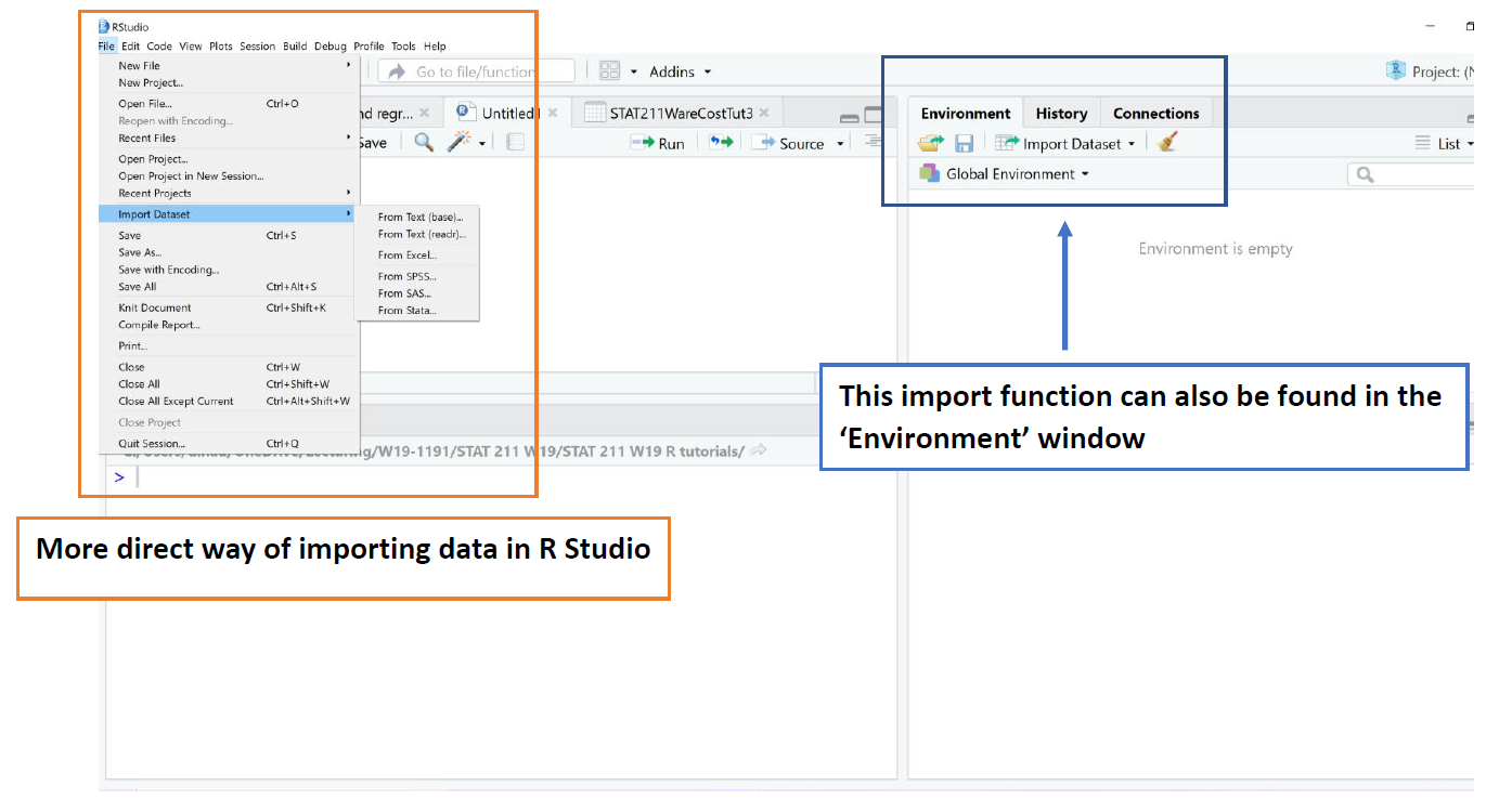
R can also import other data formats, such as excel or csv. Try looking up the functions read.csv() and read.table() using instruction from Section A.4.2.

Figure A.2: Importing Datasets in RStudio
A.8.3 Working Directory
Your data file can be anywhere in the computer. To load the file correctly you need to specify the directory where the file is saved. For example, if it is saved in drive C:
To use this command
i.e., to load the data without specifying the full directory, you need to set the working directory to be same as the directory where the file is saved. You can set the working directory using one of these ways
In RStudio along the top bar choose Session > Set Working Directory > Choose Directory
Use the function
getwd()to see what the current working directory (wd) is and usesetwd()to set a new working directory. For example
Now, if you go to the Files tab, you can see all the files in your directory. One tip is to (i) save your .R or .Rmarkdown file and the data set in the same folder and then (ii) open a new RStudio window by opening .R or .Rmarkdown file from that folder. This way, the default working directory will be the directory your files are stored. It’s also easier to manage all your files in one folder.
A.8.4 Extracting Elements from a Data Frame
You can use the column names of a data frame as defined objects in the Environment by attaching the data frame to R
For example, the data frame mydata has column Gender. After attaching mydata, we can work with column Gender directly as a saved vector in R.
## [1] "M" "F" "M" "F" "M"Once you have completed work with the data set, you can detach them from use
If you do not want to attach the data set, you can call the column (variable) using the $ operator
## [1] "M" "F" "M" "F" "M"Exercise A.2 How many people are in the mydata dataset? What is the sum of their heights?
Notes: To learn more about R, visit https://libraryguides.mcgill.ca/R.