5 Normal Distribution
In the Chapter 4, we learn about random variables and their probability functions. We discuss the Bernoulli distribution and Continuous uniform distribution as examples of discrete and continuous distributions. In this lesson, we discuss normal distribution, a continuous distribution that plays the most important role in statistics.
5.1 Normal Distribution
5.1.1 Probability Density Function
A random variable \(X\) is said to follow a normal distribution (or Gaussian distribution) if it has the probability density function of the form \[f(x) = \frac{1}{\sqrt{2\pi}\sigma}e^{-\frac{1}{2}\left(\frac{x-\mu}{\sigma}\right)^2}, \hspace{10mm} \text{for } x \in (-\infty, \infty)\] where \(-\infty < \mu < \infty\) and \(\sigma > 0\) are two parameters of this distribution.
We denote \(X \sim \mathcal{N}(\mu, \sigma^2)\), meaning that \(X\) follows a normal distribution with parameters \(\mu\) and \(\sigma^2\).
5.1.2 Expected Value and Variance
If \(X \sim \mathcal{N}(\mu, \sigma^2)\), then
The mean (expected value) of \(X\) is \(\mu = \mathbb{E}(X)\)
The variance of \(X\) is \(\sigma^2 = \mathrm{var}(X)\)
So it is quite straight forward to tell the mean and variance of the \(\mathcal{N}(\mu, \sigma^2)\) distribution from the notation. In fact, \(\mu\) and \(\sigma^2\) are called parameters of the normal distribution.
5.1.3 Shape of the Distribution
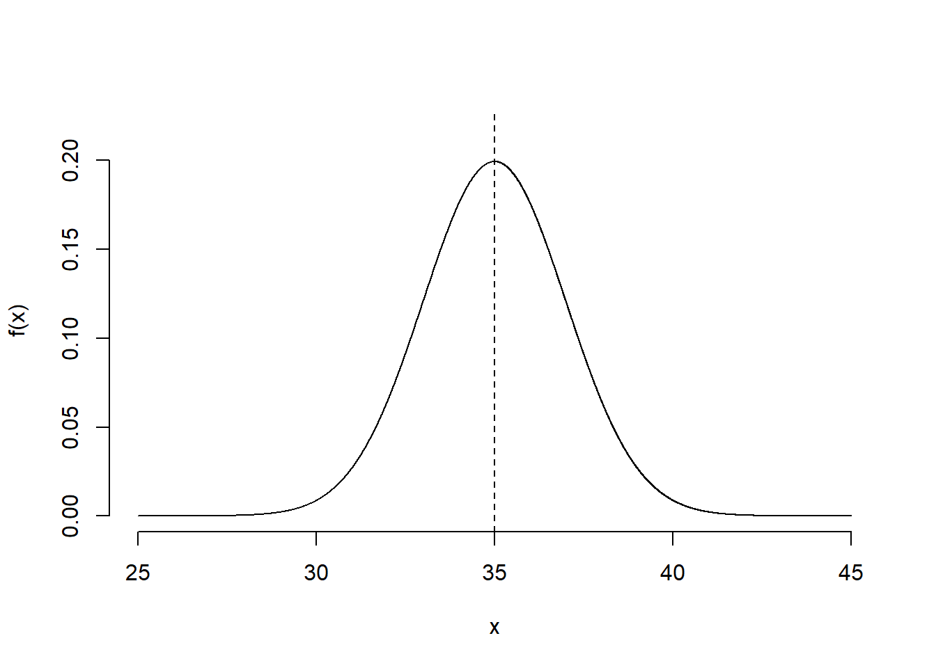
Figure 5.1: A normal distribution
The normal distribution
has a bell shape
is always symmetric about its means (creates mirror images around the mean)
the mean is called the location parameter, meaning that it controls the location of the distribution on the \(x\)-axis
the variance is called the scale parameter, meaning that it controls the spread of the distribution.
5.1.4 Effect of the mean \((\mu)\)
The mean shifts the distribution along the \(x\)-axis. Therefore it is a called the location parameter.
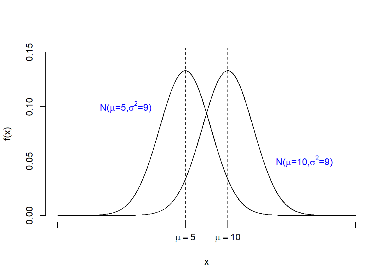
Figure 5.2: Changing \(\mu\) changes the location of the distribution
5.1.5 Effect of the Variance (\(\sigma^2\))
The variance either stretches out or pulls in the distribution. Therefore it is called the scale parameter.
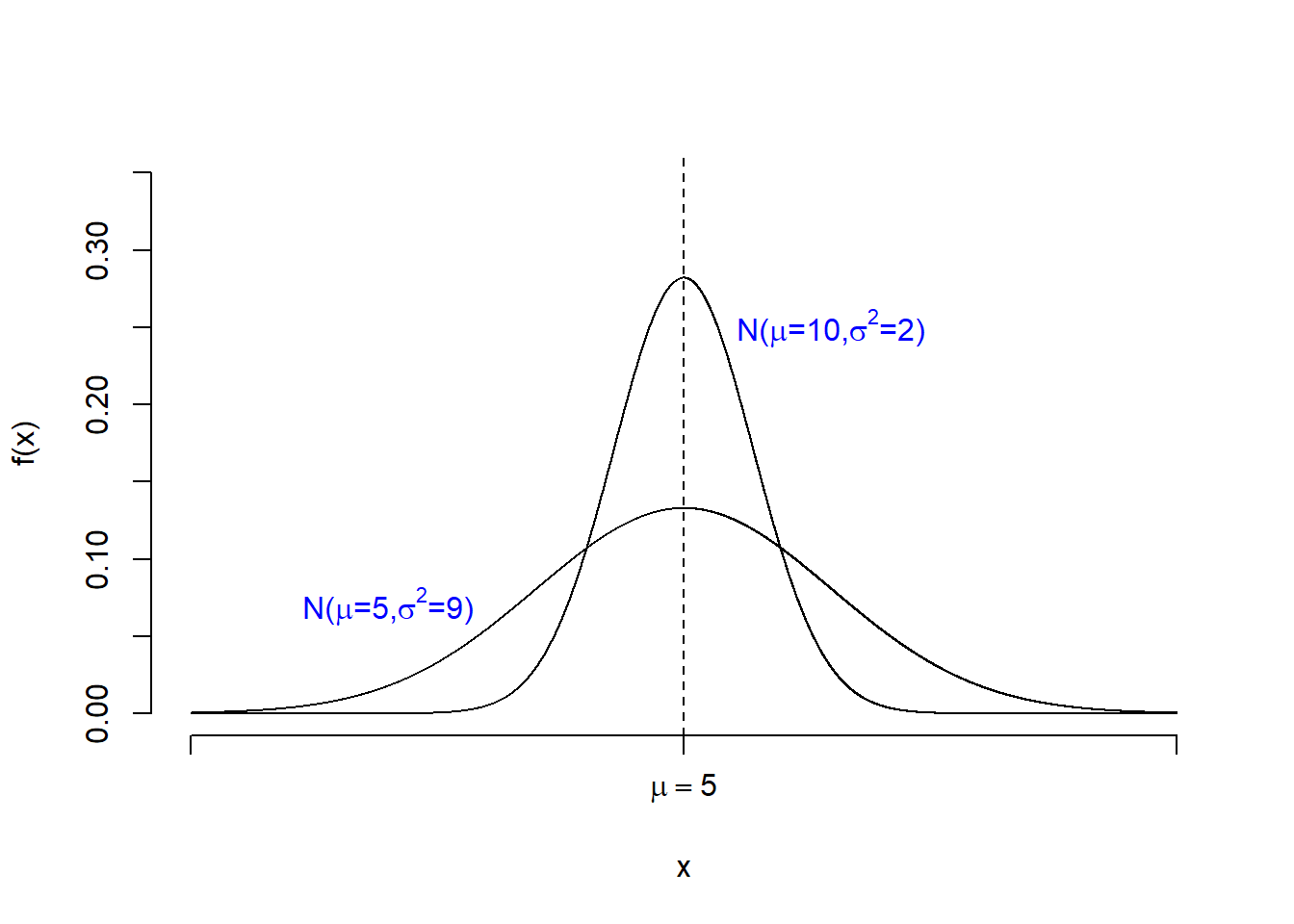
Figure 5.3: Changing \(\sigma^2\) changes the spread of the distribution
A few more examples
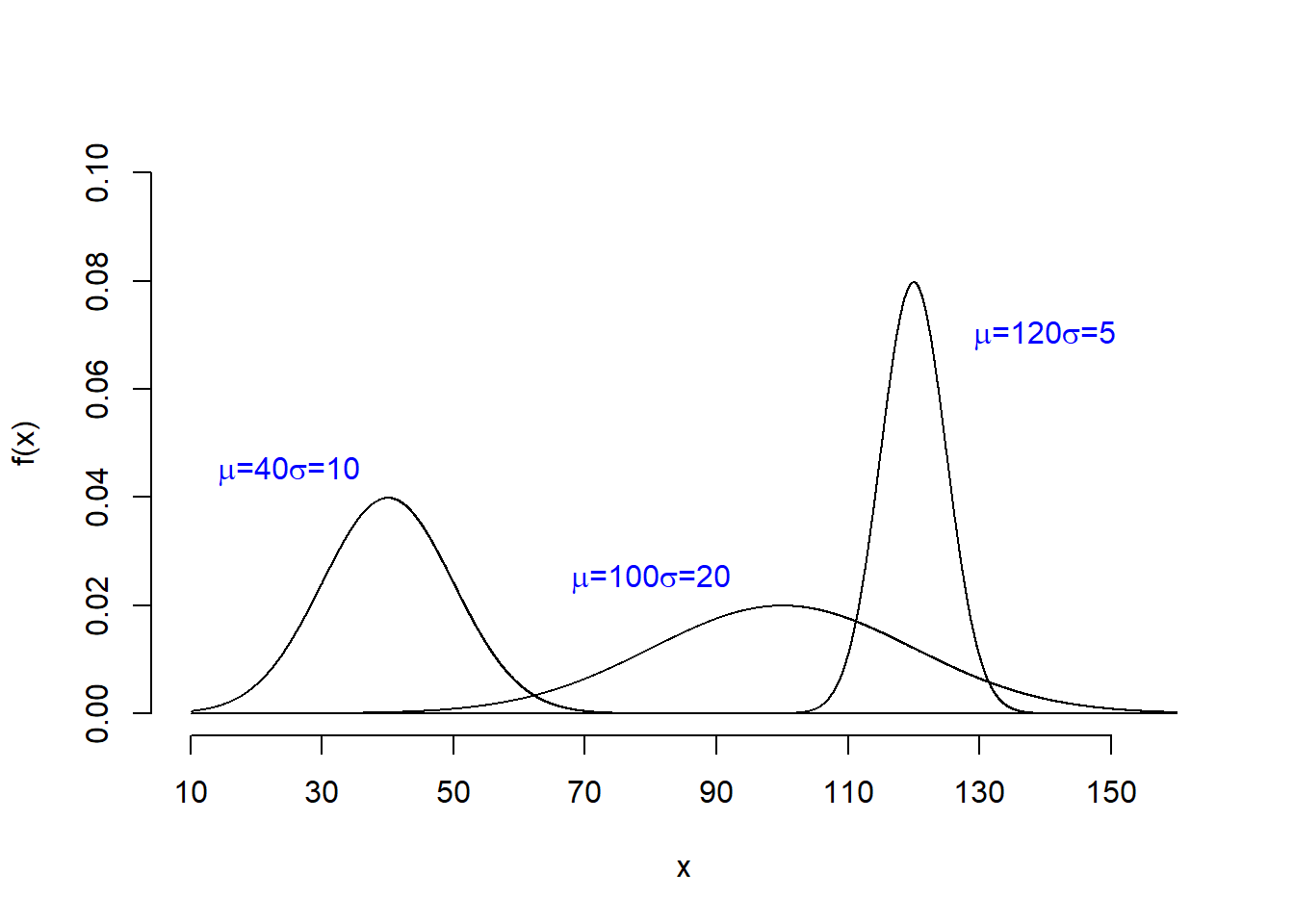
Figure 5.4: Examples of normal distribution
5.1.6 The Empirical Rule of Normal Distribution
For any normal distribution,
68% of the data will be contained within one standard deviation of the mean.
95% of the data will be contained within two standard deviations of the mean.
99.7% of the data will be contained within three standard deviations of the mean.
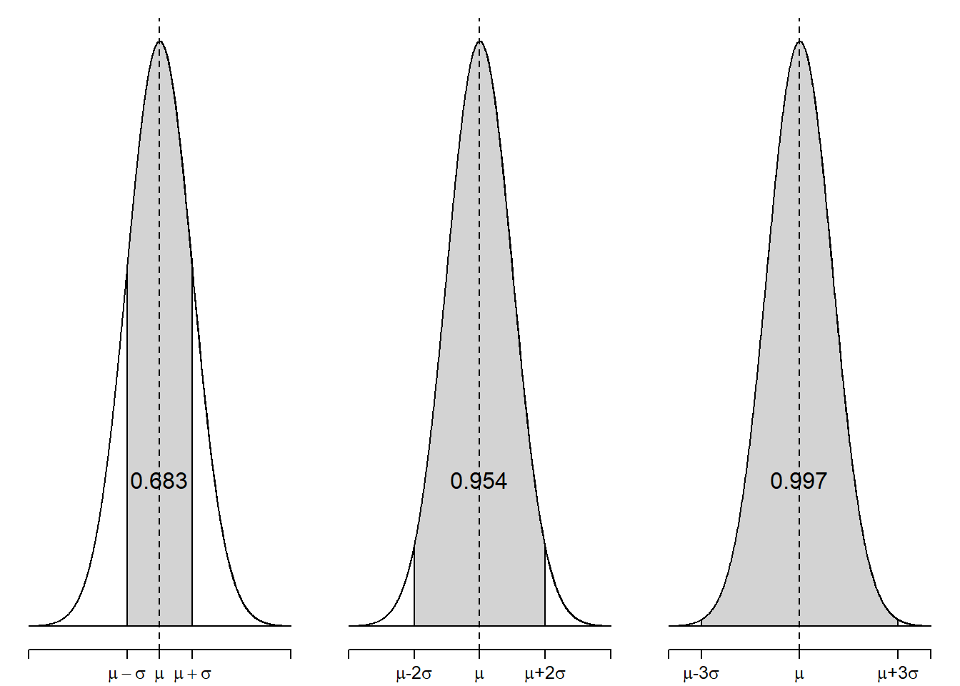
Figure 5.5: Empirical rule of standard normal distribution
5.1.7 Ubiquity of Normal Distribution
A reason why the normal distribution is so important is that the distributions of many variables in real life has bell-curve shapes which resemble the shape of normal distributions.
For example, the distribution of human’s height is roughly normally distributed. Think about it, majority of, say male, are around may be 170cm - 180 cm (about 66 to 70 inches) with less people from 160cm - 170 cm or 180 - 190 cm, and many fewer shorter than 160 cm or taller than 190 cm. This dictates a bell-curve shape for the distribution of height. The figure below shows the distribution of self-reported heights for 812 males given in the data set heights from package dslabs in R.
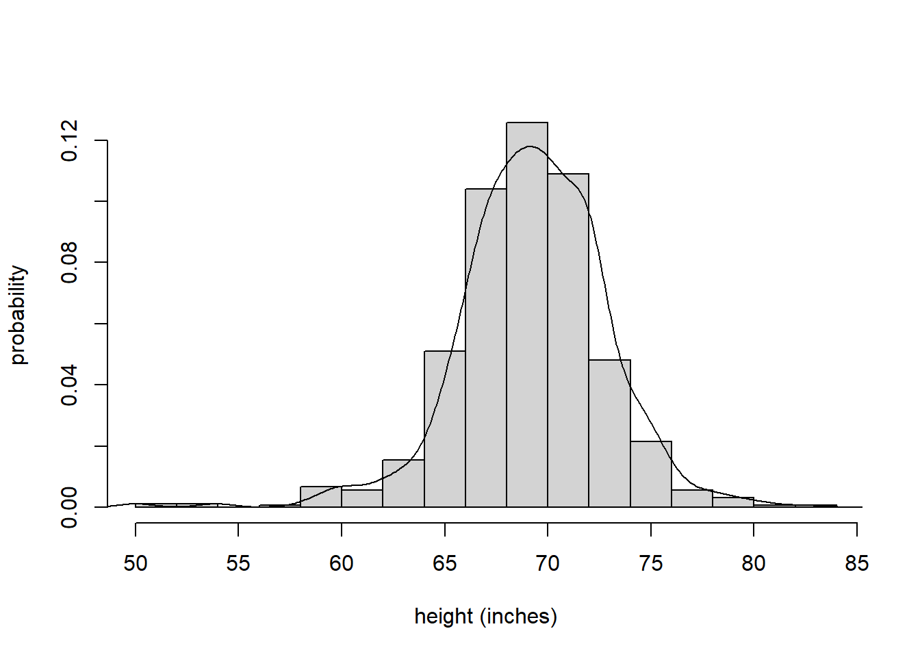
Figure 5.6: Distribution of self-reported heights for 812 males.
Another example is the one-day return of a stock. The figure below shows the distribution of Google stock’s daily return from 2005-02-07 to 2005-07-07 given in the data set google from package UsingR in R. We can see that this distribution also roughly has a bell shape curve.
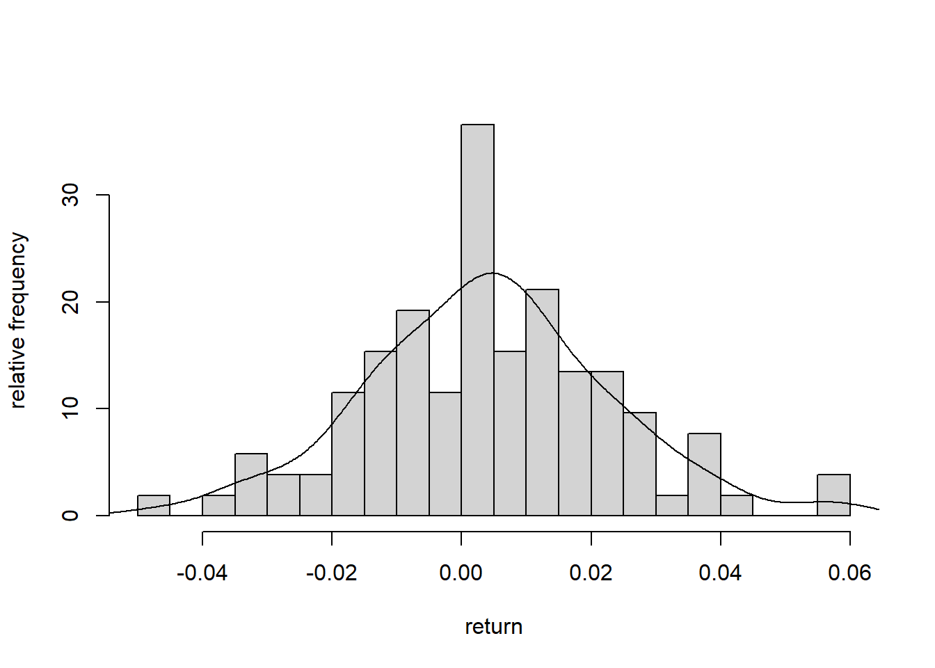
Figure 5.7: Distribution of Google stock’s daily return from 2005-02-07 to 2005-07-07.
5.2 Standard Normal Distribution
5.2.1 Probability Density Function
A normal distribution with mean of 0 (\(\mu=0\)) and variance of 1 (\(\sigma^2=1\)) is called a standard normal distribution. Notation: \(\mathcal{N}(0,1)\).
A standard normal random variable is usually denoted by \(Z\). We write \(Z\sim \mathcal{N}(0,1)\) and we say \(Z\) follows a standard normal distribution.
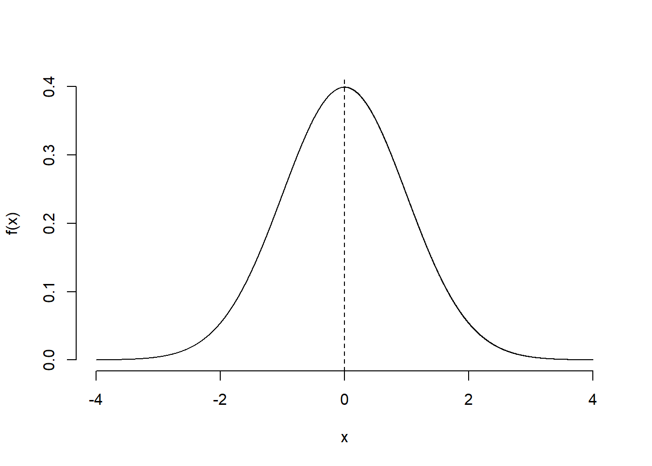
Figure 5.8: Standard normal distribution
The pdf (probability density function) of the standard normal distribution is
\[f(z) = \frac{1}{\sqrt{2\pi}}e^{-\frac{z^2}{2}}\]
From Chapter 4, we know that for any continuous random variable, to calculate the probability that the random variable lies within an interval \((a,b)\), we need to integrate the pdf from \(a\) to \(b\). Unfortunately, except for the Continuous uniform distribution we learn in 4, it is hard to calculate the integral for any continuous distributions by hand. Hence, usually we use a computer to calculate the probability, or we need to refer to a probability table.
5.2.2 \(Z\)-table
For standard normal distribution, we have the \(Z\)-table. This table provides us with the cumulative distribution, \(F(z) = \mathbb{P}(Z \le z)\), i.e., the area to the left of the observed value of \(z\).
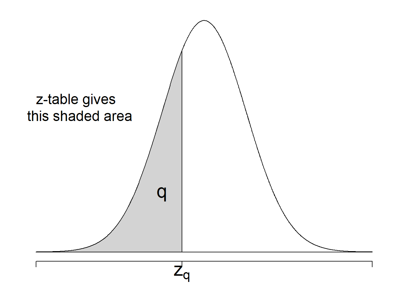
| 0.00 | 0.01 | 0.02 | 0.03 | 0.04 | 0.05 | 0.06 | 0.07 | 0.08 | 0.09 | |
|---|---|---|---|---|---|---|---|---|---|---|
| 0.00 | 0.5000 | 0.4960 | 0.4920 | 0.4880 | 0.4840 | 0.4801 | 0.4761 | 0.4721 | 0.4681 | 0.4641 |
| -0.10 | 0.4602 | 0.4562 | 0.4522 | 0.4483 | 0.4443 | 0.4404 | 0.4364 | 0.4325 | 0.4286 | 0.4247 |
| -0.20 | 0.4207 | 0.4168 | 0.4129 | 0.4090 | 0.4052 | 0.4013 | 0.3974 | 0.3936 | 0.3897 | 0.3859 |
| -0.30 | 0.3821 | 0.3783 | 0.3745 | 0.3707 | 0.3669 | 0.3632 | 0.3594 | 0.3557 | 0.3520 | 0.3483 |
| -0.40 | 0.3446 | 0.3409 | 0.3372 | 0.3336 | 0.3300 | 0.3264 | 0.3228 | 0.3192 | 0.3156 | 0.3121 |
| -0.50 | 0.3085 | 0.3050 | 0.3015 | 0.2981 | 0.2946 | 0.2912 | 0.2877 | 0.2843 | 0.2810 | 0.2776 |
| -0.60 | 0.2743 | 0.2709 | 0.2676 | 0.2643 | 0.2611 | 0.2578 | 0.2546 | 0.2514 | 0.2483 | 0.2451 |
| -0.70 | 0.2420 | 0.2389 | 0.2358 | 0.2327 | 0.2296 | 0.2266 | 0.2236 | 0.2206 | 0.2177 | 0.2148 |
| -0.80 | 0.2119 | 0.2090 | 0.2061 | 0.2033 | 0.2005 | 0.1977 | 0.1949 | 0.1922 | 0.1894 | 0.1867 |
| -0.90 | 0.1841 | 0.1814 | 0.1788 | 0.1762 | 0.1736 | 0.1711 | 0.1685 | 0.1660 | 0.1635 | 0.1611 |
| -1.00 | 0.1587 | 0.1562 | 0.1539 | 0.1515 | 0.1492 | 0.1469 | 0.1446 | 0.1423 | 0.1401 | 0.1379 |
| -1.10 | 0.1357 | 0.1335 | 0.1314 | 0.1292 | 0.1271 | 0.1251 | 0.1230 | 0.1210 | 0.1190 | 0.1170 |
| -1.20 | 0.1151 | 0.1131 | 0.1112 | 0.1093 | 0.1075 | 0.1056 | 0.1038 | 0.1020 | 0.1003 | 0.0985 |
| -1.30 | 0.0968 | 0.0951 | 0.0934 | 0.0918 | 0.0901 | 0.0885 | 0.0869 | 0.0853 | 0.0838 | 0.0823 |
| -1.40 | 0.0808 | 0.0793 | 0.0778 | 0.0764 | 0.0749 | 0.0735 | 0.0721 | 0.0708 | 0.0694 | 0.0681 |
| -1.50 | 0.0668 | 0.0655 | 0.0643 | 0.0630 | 0.0618 | 0.0606 | 0.0594 | 0.0582 | 0.0571 | 0.0559 |
| -1.60 | 0.0548 | 0.0537 | 0.0526 | 0.0516 | 0.0505 | 0.0495 | 0.0485 | 0.0475 | 0.0465 | 0.0455 |
| -1.70 | 0.0446 | 0.0436 | 0.0427 | 0.0418 | 0.0409 | 0.0401 | 0.0392 | 0.0384 | 0.0375 | 0.0367 |
| -1.80 | 0.0359 | 0.0351 | 0.0344 | 0.0336 | 0.0329 | 0.0322 | 0.0314 | 0.0307 | 0.0301 | 0.0294 |
| -1.90 | 0.0287 | 0.0281 | 0.0274 | 0.0268 | 0.0262 | 0.0256 | 0.0250 | 0.0244 | 0.0239 | 0.0233 |
| -2.00 | 0.0228 | 0.0222 | 0.0217 | 0.0212 | 0.0207 | 0.0202 | 0.0197 | 0.0192 | 0.0188 | 0.0183 |
| -2.10 | 0.0179 | 0.0174 | 0.0170 | 0.0166 | 0.0162 | 0.0158 | 0.0154 | 0.0150 | 0.0146 | 0.0143 |
| -2.20 | 0.0139 | 0.0136 | 0.0132 | 0.0129 | 0.0125 | 0.0122 | 0.0119 | 0.0116 | 0.0113 | 0.0110 |
| -2.30 | 0.0107 | 0.0104 | 0.0102 | 0.0099 | 0.0096 | 0.0094 | 0.0091 | 0.0089 | 0.0087 | 0.0084 |
| -2.40 | 0.0082 | 0.0080 | 0.0078 | 0.0075 | 0.0073 | 0.0071 | 0.0069 | 0.0068 | 0.0066 | 0.0064 |
| -2.50 | 0.0062 | 0.0060 | 0.0059 | 0.0057 | 0.0055 | 0.0054 | 0.0052 | 0.0051 | 0.0049 | 0.0048 |
| -2.60 | 0.0047 | 0.0045 | 0.0044 | 0.0043 | 0.0041 | 0.0040 | 0.0039 | 0.0038 | 0.0037 | 0.0036 |
| -2.70 | 0.0035 | 0.0034 | 0.0033 | 0.0032 | 0.0031 | 0.0030 | 0.0029 | 0.0028 | 0.0027 | 0.0026 |
| -2.80 | 0.0026 | 0.0025 | 0.0024 | 0.0023 | 0.0023 | 0.0022 | 0.0021 | 0.0021 | 0.0020 | 0.0019 |
| -2.90 | 0.0019 | 0.0018 | 0.0018 | 0.0017 | 0.0016 | 0.0016 | 0.0015 | 0.0015 | 0.0014 | 0.0014 |
| -3.00 | 0.0013 | 0.0013 | 0.0013 | 0.0012 | 0.0012 | 0.0011 | 0.0011 | 0.0011 | 0.0010 | 0.0010 |
| -3.10 | 0.0010 | 0.0009 | 0.0009 | 0.0009 | 0.0008 | 0.0008 | 0.0008 | 0.0008 | 0.0007 | 0.0007 |
| -3.20 | 0.0007 | 0.0007 | 0.0006 | 0.0006 | 0.0006 | 0.0006 | 0.0006 | 0.0005 | 0.0005 | 0.0005 |
| -3.30 | 0.0005 | 0.0005 | 0.0005 | 0.0004 | 0.0004 | 0.0004 | 0.0004 | 0.0004 | 0.0004 | 0.0003 |
| -3.40 | 0.0003 | 0.0003 | 0.0003 | 0.0003 | 0.0003 | 0.0003 | 0.0003 | 0.0003 | 0.0003 | 0.0002 |
Using the fact that standard normal distribution is symmetric round 0 and the total area under the curve is 1, we can use the numbers from the table to solve for the probability of any interval that we may want.
Example 5.1 Find that probability that
\(Z < -1.37\)
\(Z > 1.5\)
\(-1 < Z < 1.15\)
\(|Z| > 0.5\)
Find the \(z\) value that corresponds to the highest 20%
Find the \(z\) value that corresponds to the lowest 3% (i.e., \(3\)rd percentile)
Find the \(z\) value that corresponds to the 95% percentile
Solution:
To find \(\mathbb{P}(Z < -1.37)\), we first look at the leftmost column, and find the row -1.30. Then we follow this row and look at column 0.07. The element in this cell is 0.0853. So \[\mathbb{P}(Z < -1.37) = \mathbb{P}(Z \le -1.37) = 0.0853\]
Because the standard normal distribution is symmetric around 0, we have \[\mathbb{P}(Z > 1.5) = \mathbb{P}(Z < -1.5) = 0.0668\].
\[\begin{align*} \mathbb{P}(-1 < Z < 1.15) & = \mathbb{P}(Z < 1.15) - \mathbb{P}(Z \le -1) \\ & = \mathbb{P}(Z > -1.15) - \mathbb{P}(Z < -1) \\ & = (1 - \mathbb{P}(Z < -1.15)) - \mathbb{P}(Z < -1) \\ & = (1 - 0.1251) - 0.1587 = 0.7162 \end{align*}\]
\[\begin{align*} \mathbb{P}(|Z| > 0.5) & = \mathbb{P}(Z > 0.5) + \mathbb{P}(Z < -0.5) \\ & = \mathbb{P}(Z < -0.5) + \mathbb{P}(Z < -0.5) \\ & = 2\mathbb{P}(Z < -0.5) \\ & = 2\times 0.3085 = 0.6170. \end{align*}\]
\(\mathbb{P}(Z > z) = 0.2\) so \(\mathbb{P}(Z < -z) = 0.2\).
Now we look at the \(Z\)-table and find the cell that has value \(0.2\). The cell \(-0.84\) has value \(0.2005\), which is closest to \(0.2\). So \(-z = -0.84\) and \(z = 0.84\).
\(\mathbb{P}(Z < z) = 0.03\).
The cell \(-1.88\) has value \(0.0301\) is closest to 0.03, so \(z = -1.88\).
\(\mathbb{P}(Z < z) = 0.95\) so \(\mathbb{P}(Z < -z) = 0.05\).
Now cell \(-1.64\) has value \(0.0505\) and cell \(-1.65\) has value \(0.0495\) both close to \(0.05\). We then take the average of the two cells \[-z = \frac{-1.64-1.65}{2} = -1.645 \hspace{5mm} \Rightarrow \hspace{5mm} z = 1.645.\]
Notes: The given \(Z\)-table has only negative values of \(z\) and probability values less than 0.5. So when looking for positive \(z\) or probability more than \(0.5\), we can use the following properties:
complememnt: \(\mathbb{P}(Z > z) = 1-\mathbb{P}(Z \le z)\).
\(\mathbb{P}(a < Z \le b) = \mathbb{P}(Z \le b) - \mathbb{P}(Z \le a)\).
symmetry around 0: \(\mathbb{P}(Z < z) = \mathbb{P}(Z > -z)\)
Note that
The first and the second property is true for any probability function, even for discrete probability mass function.
As we discuss in Chapter 4, for continuous random variable, \(\mathbb{P}(X = x) = 0\), so \(<\) and \(\le\) can be used interchangeably for continuous random variable. Same for \(>\) and \(\ge\).
The third property is true for only distributions that are symmetric around 0.
5.3 \(Z\)-score
5.3.1 Linearity of Normal Distribution
In Chapter 4, we learn the two properties of expectation: \[\begin{align*} \mathbb{E}(a + bX) & = a + b\mathbb{E}(X) \\ \mathrm{var}(a + bX) & = b^2\mathrm{var}(X) \end{align*}\] for constants \(a\) and \(b\). So, if \(X\) has mean \(\mu\) and variance \(\sigma^2\) and \(Y = aX + b\) then \[\mathbb{E}[Y] = a + b\mu \hspace{5mm} \text{and} \hspace{5mm} \mathrm{var}(Y) = b^2\sigma^2\] This means if we know the mean and variance of \(X\), we know the mean and variance of \(Y\). However, we may not know the distribution of \(Y\).
However, there is a special property of the normal distribution, called the linearity of normal distribution, that says \[\text{If } X \sim \mathcal{N}(\mu, \sigma^2) \hspace{5mm} \text{ then } \hspace{5mm} Y = a + bX \sim \mathcal{N}(a + b\mu, b^2\sigma^2) \] So a linear transformation of a normal distribution is another normal distribution with the mean and the variance calculated based on the linearity property of expectation.
5.3.2 \(Z\)-score
In the above linearity property of normal distribution, if we let \(a = -\frac{\mu}{\sigma}\) and \(b = \frac{1}{\sigma}\), then
\[\text{If } X \sim \mathcal{N}(\mu, \sigma^2) \hspace{5mm} \text{ then } \hspace{5mm} Z = \frac{X-\mu}{\sigma} \sim \mathcal{N}(0, 1)\]
\(Z = \frac{X-\mu}{\sigma}\) is called the \(Z\)-score of \(X\) and \(X\) is said to be standardized to be \(Z\).
So, any normal distribution can be transformed into a standard normal distribution by standardizing them into a \(Z\)-score. This is extremely helpful when we calculate the probabilities for we normal random variables, because we do not need to do integration for every different normal distribution with different \(\mu\) and \(\sigma^2\). I will illustrate this with examples in the next section.
5.3.3 Examples
Example 5.2 Suppose the random variable \(X\) has a normal distribution with a mean of \(\mu = 120\) and a standard deviation of \(\sigma = 20\). Find
\(\mathbb{P}(X < 105)\)?
\(\mathbb{P}(92 < X < 108)\)?
\(\mathbb{P}(X = 84)\)?
The interquartile range of the distribution of \(X\)?
Solution: \(X \sim \mathcal{N}(\mu = 120, \sigma^2 = (20)^2)\)
\[\begin{align*} \mathbb{P}(X < 105) & = \mathbb{P}\left(\frac{X-\mu}{\sigma} < \frac{105-\mu}{\sigma}\right) \\ & = \mathbb{P}\left(Z < \frac{105-120}{20}\right) \\ & = \mathbb{P}(Z < -0.75) = 0.2266 \end{align*}\]
\[\begin{align*} \mathbb{P}(92 < X < 108) & = \mathbb{P}\left(\frac{92-120}{20} < Z < \frac{108-120}{20}\right) \\ & = \mathbb{P}(-1.4 < Z < -0.6) \\ & = \mathbb{P}(Z < -0.6) - \mathbb{P}(Z < -1.4) \\ & = 0.2743 - 0.0808 = 0.1935 \end{align*}\]
\(\mathbb{P}(X = 84) = 0\) since \(X\) is a continuous random variable.
Recall that \(IQR = Q3 - Q1\). Now Q1 is the 0.25 quantile and Q1 is the 0.75 quantile.
\(\mathbb{P}(Z < z) = 0.25\). Because the cell \(-0.67\) is \(0.2514\) and the cell \(-0.68\) is \(0.2483\) both close to 0.25, then \[z = \frac{-0.67-0.68}{2} = -0.675\]
\(\mathbb{P}(Z < z) = 0.75\) so \(\mathbb{P}(Z > -z) = 0.75\).
Then \(\mathbb{P}(Z < -z) = 0.25\). So \(-z = -0.675\) from above and \(z = 0.675\)
Q1 for \(X\) is \(-0.675 \times 20 + 120 = 106.5\).
Q3 for \(X\) is \(0.675 \times 20 + 120 = 133.5\)
The IQR for distribution of \(X\) is \(Q3-Q2 = 133.5-106.5 = 27\) 16.
Example 5.3 Suppose the students’ rent is normally distributed with mean price of \(800\) dollars and standard deviation of \(100\) dollars.
What fraction of the rent will be within one standard deviation from the mean?
What price range will the middle \(80\%\) of the prices lie between?
What fraction of the price is more than \(\$900\)?
Suppose school has some subsidy for students’ rent. How much should school give to each student so that less than \(5\%\) of students pay more than \(900\) dollars?
Without the subsidy, how much the standard deviation should be so that less than \(5\%\) of students pay more than \(900\) dollars?
Solution: Let \(X\) be the student’s rent. Then \(X \sim \mathcal{N}(\mu = 800, \sigma^2 = (100)^2)\)
\[\begin{align*} \mathbb{P}(800-100 < X < 800+100) & = \mathbb{P}(700 < X < 900) \\ & = \mathbb{P}\left(\frac{700-\mu}{\sigma} < \frac{X - \mu}{\sigma} < \frac{900-\mu}{\sigma} \right) \\ & = \mathbb{P}\left(\frac{700-800}{100} < Z < \frac{900-800}{100}\right) \\ & = \mathbb{P}(-1<Z<1) \\ & = \mathbb{P}(Z < 1) - \mathbb{P}(Z < -1) \\ & = \mathbb{P}(Z > -1) - \mathbb{P}(Z < -1) \\ & = (1 - \mathbb{P}(Z < -1)) - \mathbb{P}(Z < -1) \\ & = 1 - 2\times \mathbb{P}(Z < -1) \\ & = 1 - 2\times 0.1587 = 0.6826 \end{align*}\]
The interval covers \(80\%\). Therefore \[\mathbb{P}(a < X < b) = 0.8 \hspace{5mm} \Rightarrow \hspace{5mm} \mathbb{P}\left(\frac{a-800}{100} < Z < \frac{b-800}{100}\right) = 0.8 \]
Now, because this is the middle \(80\%\), so the interval should be symmetric around the mean. Hence, \[- \frac{a-800}{100} = \frac{b-800}{100}\] Let \(z = \frac{b-800}{100}\). We have \[\begin{align*} \mathbb{P}(-z < Z < z) = 0.8 & = \mathbb{P}(Z < z) - \mathbb{P}(Z < -z) \\ & = \mathbb{P}(Z > -z) - \mathbb{P}(Z < -z) \\ & = (1 - \mathbb{P}(Z < -z)) - \mathbb{P}(Z < -z) \\ & = 1 - 2\times\mathbb{P}(Z < -z) \\ 0.1 & = \mathbb{P}(Z < -z) \end{align*}\] From the table, \(-z = -1.28\). Now \[\frac{b-800}{100} = 1.28 \Rightarrow b = 928\] \[\frac{a-800}{100} = -1.28 \Rightarrow a = 672\] So the middle \(80\%\) of the rent price falls between \(672\) and \(928\) dollars.
\(\mathbb{P}(X > 900) = \mathbb{P}\left(Z > \frac{900-800}{100}\right) = \mathbb{P}(Z > 1) = \mathbb{P}(Z < -1) = 0.1587\).
We want \(\mathbb{P}(X > 900) < 0.05\). If school gives each student \(x\) dollars for rent, the mean rent to be paid will decrease by \(x\) dollars. This means \[\begin{align*} \mathbb{P}\left(Z > \frac{900 - (800-x)}{100}\right) & < 0.05 \\ \Rightarrow \mathbb{P}\left(Z < \frac{(800-x)-900}{100}\right) & < \mathbb{P}(Z < -1.645) \\ \Rightarrow \frac{(800-x)-900}{100} & < -1.645 \\ \Rightarrow x > 64.5 \end{align*}\] So school needs to give each student at least 64.5 dollars.
We want to find a new standard deviation. Suppose it is \(x\). Then \[\begin{align*} \mathbb{P}\left(Z > \frac{900 - 800}{x}\right) & < 0.05 \\ \Rightarrow \mathbb{P}\left(Z < \frac{800-900}{x}\right) & < \mathbb{P}(Z < -1.645) \\ \Rightarrow \frac{(800-900}{x} & < -1.645 \\ \Rightarrow x < 60.79 \end{align*}\] So the standard deviation has to be at most 60.79 dollars.
Exercise 5.1 Verify the empirical rule of normal distribution. Hint: Look at part a of Example 5.3.
5.4 Calculate Normal Probabilities in R
We can also skip looking at the \(Z\)-table and directly calculate normal probabilities in R.
To calculate \(Z\)-probabilities in R, we use two functions pnorm() and qnorm(). The function pnorm(a) will give you the probability \(\mathbb{P}(Z < a)\) for any number \(a\). For example,
## [1] 0.9772499is the probability \(\mathbb{P}(Z < 2)\).
The function qnorm(q) will give you the number \(a\) that satisfy \(\mathbb{P}(Z < a) = q\). For example,
## [1] 0.6744898tells us that \(\mathbb{P}(Z < 0.674) = 0.75\).
Besides \(Z\), you can also calculate similar probabilities for \(X \sim \mathcal{N}(\mu, \sigma^2)\) by specifying arguments \(\mu\) and \(\sigma\) to parameters mean and sd of the two functions pnorm() and qnorm(). For example,
## [1] 0.6914625is the probability \(\mathbb{P}(X < 2)\) if \(X \sim \mathcal{N}(1, 2^2)\).
Notes: In this Chapter, we focus only on the normal distribution. The reason is that it is the most important distribution in statistics! The problems related to this lesson can be new and challenging. But again there is no short cut but to practice and practice! Try to practice looking up the \(Z\)-table, and work out the examples and exercises in this lesson by yourself.
Alternative solution: IQR for \(Z\) is \(0.675 - (-0.675) = 1.35\). So IQR for \(X\) is \(1.35*20 = 27\). You don’t need to add 120 because when we subtract Q1 from Q3, 120 got canceled.↩︎