4 Random Variables

At the end of Chapter 3, we discussed that: in the tree diagram examples, each node is a categorical variable and the branches are events corresponding to categories of the variable. However, in Chapter 3, we focused more on events rather than the variables. In this lesson, we will discuss in more detail about variables in the context of probability. We will also learn the concepts of probability function and expectation.

4.1 Random Variables

4.1.1 What is A Random Variable?

Random variable is a function that assigns a value to each of an experiment’s outcomes. Since the value of a random variable is directly related to the outcome of a probabilistic experiment, the value of the random variable is random, i.e., not pre-determined.

Example 4.1 Probabilistic experiment: roll a six-sided die.

Outcome	Number appear	Is odd? (\(1\) yes, \(0\) no)	Is divisible by \(3\)? (\(1\) yes, \(0\) no)
\(1\)	\(1\)	\(1\)	\(0\)
\(2\)	\(2\)	\(0\)	\(0\)
\(3\)	\(3\)	\(1\)	\(1\)
\(4\)	\(4\)	\(0\)	\(0\)
\(5\)	\(5\)	\(1\)	\(0\)
\(6\)	\(6\)	\(0\)	\(1\)

Whether the number obtained is odd, and whether the number obtained is divisible by 3 are both random variables because they give some values to each possible outcome of the probabilistic experiment.

Example 4.2 Probabilistic experiment: randomly pick a person on the street and ask for their information

Outcome	Age	Height (cm)	Gender
Person A	25	\(164.4\)	Female
Person B	36	\(173.3\)	Male
Person C	49	\(188.1\)	Others
Person D	53	\(157.8\)	Female
\(\vdots\)	\(\vdots\)	\(\vdots\)	\(\vdots\)

The above table lists all people I could have picked on the street, i.e., all the possible outcome of the experiment. So age, height and gender are random variables because they return specific values for each possible person I could have picked.

Example 4.3 My own age is a variable because its value changes year by year. But it is is not a random variable, because its value is not random nor does it relate to any probabilistic experiment.

Notes: From the examples above, we see that

• There can be more than one random variables for one probabilistic experiment

• A random variable can be numeric (quantitative) or categorical (qualitative)

• A random variable can take finite or infinite number of possible values.

• The set of possible values that a random variable can take may be different from the sample space of the probabilistic experiment.

4.1.2 Observed Values

In Chapter 3, we learn that a probabilistic experiment is a process that is repeatable, and every repetition of the probabilistic experiment is called a run or a trial. Now, it is important to differentiate the (unknown) general value of a random variable in the probabilistic experiment and the (known) value of the random variable in a specific run.

• Random variable: the unknown and general variable that represents an outcome of a probabilistic experiment

  • often denoted by capitalized letters, for example \(X, Y, Z\), etc.

• Observed value: the known value of the random variable as a result of a specific run of the probabilistic experiment

  • often denoted by lower-case letters, for example, \(x, y, z\), etc.

  • observed data: a collection of observed values.

Example 4.4 In Example 4.1, the number obtained from rolling a fair six-sided die is a random variable, say \(X\). \(X\) can take values \(1, 2, 3, 4, 5, 6\).

Suppose today at this time I roll a die and obtain \(3\). Then this number \(3\) is an observed value of \(X\). Now, if I repeat rolling the die for \(15\) minutes and obtain the results \[6, 1, 1, 3, 2, 5, 4, 5, 2, 6, 1, 4, 5, 6, 4, 6, 5, 6, 2, 1, 4, 4, 4, 5, 6, ...\] then these are called the observed data of the random variable \(X\).

4.1.3 Defining Probabilities and Events with Random Variables

Since random variables are directly related to the outcome of a probabilistic experiment, we can use random variables to define events of the probabilistic experiment. In fact, it is often more convenient to do so, compared to the way of defining an event by listing all the outcomes in that event, especially when the sample space is very large.

Example 4.5 Some examples about using random variables to define events.

• Probabilistic experiment: rolling a six-sided die.

  • Sample space: \(\Omega = \{1,2,3,4,5,6\}\)

  • \(X\): the number obtained.

    • \(X < 4\) represents the event \(\{1,2,3\}\)

  • \(Y\): whether the number is divisible by three, 1 for yes and 0 for no.

    • \(Y = 0\) represents the event \(\{1,2,4,5\}\)

• Probabilistic experiment: tossing two coins.

  • Sample space: \(\Omega = \{HH, HT, TH, TT\}\)

  • \(X\): the outcome obtained.

    • \(X \in \{HT, TH\}\) represents the event \(\{HT, TH\}\).

  • \(Y\): the number of heads

    • \(Y = 2\) represents the event \(\{HH\}\)

    • \(Y = 1\) and \(X \in \{HT, TH\}\) both represent the event \(\{HT, TH\}\)

• Probabilistic experiment: picking a random person on street.

  • sample space: all the people walking on the street that day

  • \(X\): their age

    • \(X > 18\) represents the event that the person I picked is at least 19 years old.

    • We cannot list all the possible people walking on the street that day who are at least 19 years old to define the event. So it is more convenient to define the event with the random variable \(X\).

Exercise 4.1 Consider rolling a six-sided die. Let \(Y\) be the random variable that \[Y = \begin{cases} 0 & \text{if the number obtained is even} \\ 1 & \text{if the number obtained is odd} \end{cases}\]

1. Define the event \(Y = 0\) by listing all the possible outcomes in the event.

2. Define the event \(Y = 1\) by listing all the possible outcomes in the event.

In Chapter 3, we talk about probability as a function of a set of possible outcomes, for example, probability of the sample space (\(\mathbb{P}(\Omega) = 1\)) and probability of an event \(A\) (\(\mathbb{P}(A)\)). Now, we learn that we can use a random variable to define different events of a probabilistic experiment. Thus, we can incorporate random variables into our probability notation.

Example 4.6 Consider rolling a six-sided die. Let \(X\) be the number obtained. The probability of obtaining a number that is less than three can be denoted as \[\mathbb{P}(\{1,2\}) = \mathbb{P}(X \in \{1,2\}) = \mathbb{P}(X < 3)\]

In Example 4.1, if the die is fair, what is \(\mathbb{P}(X < 3)\)?

4.1.4 Types of Random Variables

There are two types of random variables:

• Discrete random variable: a random variable whose set of possible values are countable.

• Continuous random variables: a random variable whose set of possible values are uncountable.

The word countable comes from pure mathematics, thus the definition of countability may seem technical and we will not deal with the detail of it in this book. But informally, a set is countable if we can count the elements together with integers, say 1, 2, 3, …

Example 4.7 Examples of discrete and continuous random variables:

• \(X\): the outcome of tossing a coin. Then \(X\) is discrete since we can list the possible values of \(X\) as “1. head, 2. tail”.

• \(Y\): the number of heads when tossing 25 coins. Then \(Y\) is discrete since we can list the possible values of \(Y\) as “1. 1, 2. 2, 3. 3, …”

• \(Z\): the closing price of a stock on the New York Stock Exchange on a random day. Then, the price can be any non-negative real numbers. In this case, we cannot really count all the possible values of \(Z\) together with 1, 2, 3, … and hence \(Z\) is continuous.

Notes: To decide if a random variable is continuous or discrete, use the following facts

• a finite set is countable.

• the sets (i) the set of all natural numbers \(\mathbb{N}\), (ii) the set of all integers \(\mathbb{Z}\), and the set of all rational numbers \(\mathbb{Q}\), are countable.

• \(\mathbb{R}\), the set of all real numbers, and any real intervals are uncountable.

Example 4.8 Revisit Example 4.5:

• \(X\) is discrete because its sample space is finite.

• \(Y\) is discrete because its sample space is \(\mathbb{N}\).

• \(Z\) is continuous because its sample space is \([0, +\infty)\), which is a real interval.

Notes: It is important to differentiate the set of all possible values for a random variable and the sample space of a probabilistic experiment.

Example 4.9 Consider Example 4.1.

• the sample space is \(\{1,2,3,4,5,6\}\)

• the set of all possible values for the first random variable is \(\{1,2,3,4,5,6\}\)

• the set of all possible values for both the second and third random variables is \(\{0,1\}\).

Example 4.10 Consider Example 4.2.

• the sample space is all the people I could have picked on the street

• the set of all possible values for Age is \(\{0, 1, 2, 3, ...\}\).

• the set of all possible values for Height is \((0, +\infty)\).

• the set of all possible values for Gender is \(\{female, male, others\}\)⁹

Notes: In many cases where the random variable is in fact discrete, people tend to treat the variable as if they are continuous, especially when the possible values of the variable are numbers and there are many of them. There are many technical reasons, but basically it is because it is more convenient and simple to do so. An example where discrete variables are often treated as continuous is in linear regression. We will learn about it in Chapter 10 and 11.

Example 4.11 Students’ rent is a continuous random variable because it can take any real values, for example \(\$ 861.236\).

Exercise 4.2 Is human’s height discrete or continuous, and why?

4.2 Probability Function

4.2.1 Probability Distribution

A probability distribution describes how the probabilities are like for all possible values of a random variable. Histograms (from Chapter 2) is a good way to visualize probability distributions.

Example 4.12 Let us consider again the students’ rent data in Example @ref{exm:ex-des-hist} of Chapter 2. Looking at the histogram, we can see that

• the prices range from about 300 to 1200

• the prices around 700-800 are the most probable. In fact, the probability that the rent falls between 700 to 800 is more than 0.25

• the distribution of the rent price looks symmetric

• etc.

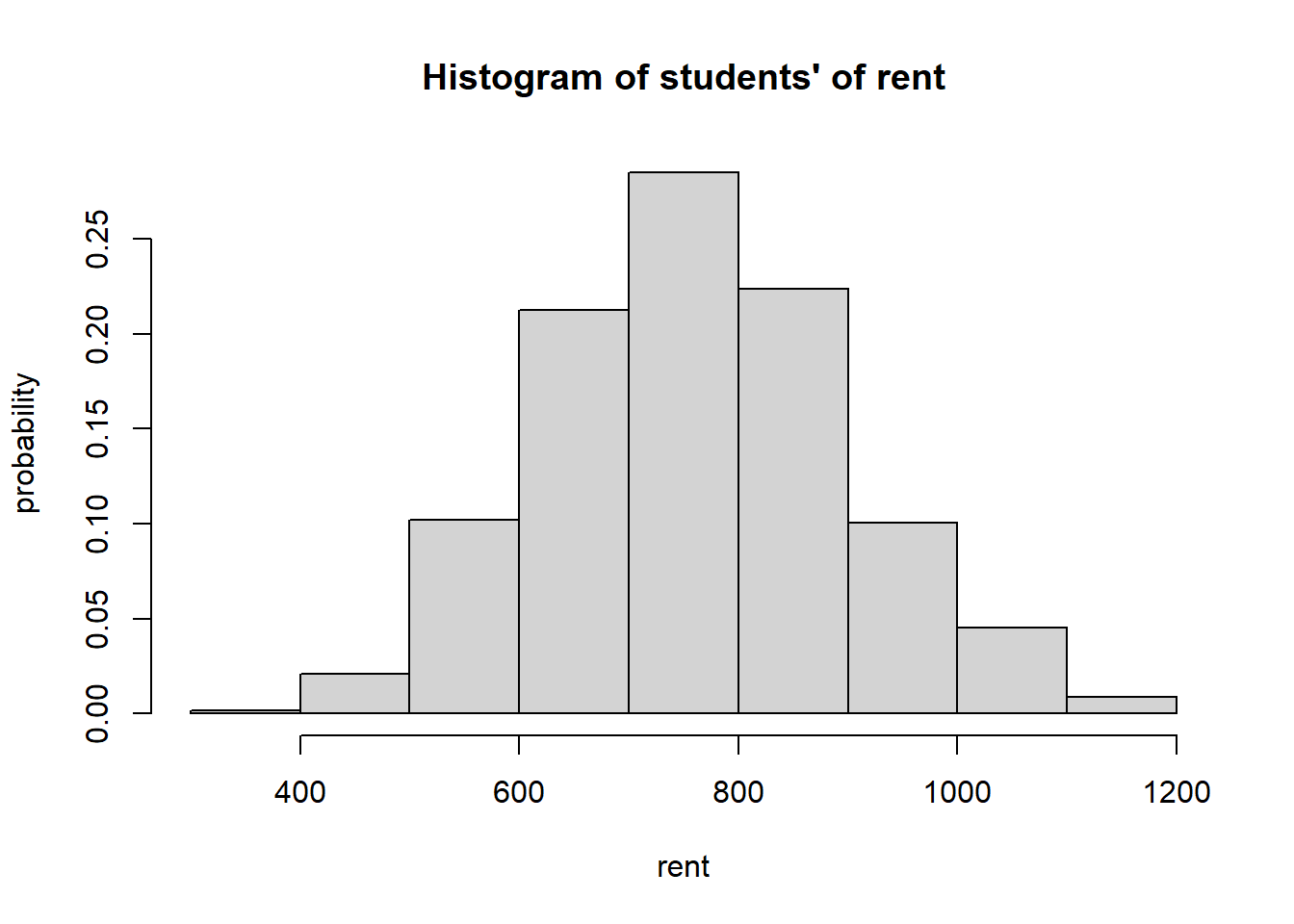
Figure 4.1: Histogram of students’ rent

Notes: Since we want to represent a probability distribution, the heights of the bars in the histogram above are standardized into relative frequencies instead of the frequencies (counts). According to the empirical view of probability we learned in Chapter 3, relative frequency can be thought of as a probability for students’ rent in the sample data.

Exercise 4.3 Verify that relative frequency satisfy the mathematical definition of a probability in Chapter 3.

4.2.2 Probability Function

Probability functions are mathematical functions that take in a possible value of a random variable, and output the probability or the probability density¹⁰ at that specific value. Therefore, they decide how probability distributions look like.

Example 4.13 Toss a fair coin. \(X\): the face obtained. The probability function is \[p(X) = \begin{cases} \frac{1}{2} & \text{if } X \text{ is head}, \\ \frac{1}{2} & \text{if } X \text{ is tail}, \\ \end{cases}\]

Exercise 4.4 Consider rolling a fair six-sided die. What is the probability function of

1. \(X\): the number obtained

2. \[Y = \begin{cases} 1 & \text{if the number obtained is less than 2} \\ 0 & \text{otherwise} \end{cases}\]

Notes: Difference between probability distributions and probability functions

• Probability distributions:

  • conceptual understanding of how the probabilities are distributed for a random variable

  • focus on the location (which values are possible), the spread (how the values are different from each other), the shape (how the probabilities are distributed among the possible values), etc.

• Probability functions:

  • mathematical functions

  • focus on the mathematical relationships/rules between a possible value of a random variable and the probability or the probability density at that value

  • decide what the probability distributions look like.

4.2.3 Discrete and Continuous Probability Functions

It is essential to note that probability functions are handled differently for discrete and continuous random variables. The reason is that is is impossible to quantify the probability that a continuous random variable obtains a specific value. More clearly,

• for example, consider the closing price of a stock in Example 4.7. This is a continuous random variable. The probability that a stock’s closing price is at 4.9375016404165072 is 0, i.e., we almost never can obtain this exact price.

• suppose on the contrary that we can assign a number for the probability of obtaining any certain value \(x\) of \(X\) to be \(k_x = \mathbb{P}(X = x) > 0\). Since there are uncountably infinitely many possible values \(x\), the sum of all these probabilities \(k_x\) will be infinite. This is contradictory to the requirement that \(\mathbb{P}(\Omega) = 1\).¹¹

• when talking about probabilities related to a continuous random variable, we usually only talk about the probabilities of intervals of possible values, for example, \(\mathbb{P}(X \le 5) = \mathbb{P}((-\infty, 5])\), or \(\mathbb{P}(1 \le X < 3) = \mathbb{P}([1,3))\) ¹² and we let \(P(X = x) = 0\) for all possible values \(x\).

This is the reason why in the definition of probability functions in Section 4.2.2, I say that a probability function takes in a possible value of the random variable and outputs the probability (for discrete random variables) or the probability density (for continuous random variables) at that specific value. We will explain more clearly what the probability density for a continuous variable is in Section 4.4. But first, let us start by considering the probability function for discrete random variables.

4.3 Probability Function for Discrete Random Variables

4.3.1 Probability Mass Function

The probability mass function (or pmf) takes in a possible value of a discrete random variable and outputs the probability of obtaining that specific value. \[p(x) = \mathbb{P}(X = x)\]

Here, \(p\) denotes the probability mass function, \(\mathbb{P}\) denotes probability in general¹³, \(X\) denotes the discrete random variable, and \(x\) denotes a specific value of \(X\).

Using the mathematical definition of probability in Section 3.1.4, we have the properties of a probability mass function \(p\)

1. \(0 \le p(x) \le 1\)

2. \(\sum_{\text{all }x}p(x) = \mathbb{P}(\Omega) = 1\).

Example 4.14 A discrete random variable \(X\) can take five possible values: \(2, 3, 5, 8\) and \(10\). Its probability mass function is given in the following table

\(x\)	\(2\)	\(3\)	\(5\)	\(8\)	\(10\)
\(p(x) = \mathbb{P}(X = x)\)	\(0.15\)	\(0.10\)	?	\(0.25\)	\(0.25\)

1. Solve for \(\mathbb{P}(X = 5)\).

2. What is the probability \(X\) equals \(2\) or \(10\)?

3. What is \(\mathbb{P}(X \le 8)\)?

4. What is \(\mathbb{P}(X < 8)\)?

Solution:

1. Since probability of the whole sample space is 1, and the probability of union of mutually exclusive events is the sum of probability of each event \[\begin{align*} \mathbb{P}(\Omega) = 1 & = \mathbb{P}(X\in\{2,3,5,8,10\}) \\ & = \mathbb{P}(X = 2) + \mathbb{P}(X = 3) + \mathbb{P}(X = 5) + \mathbb{P}(X = 8) + \mathbb{P}(X = 10) \\ & = 0.15 + 0.10 + \mathbb{P}(X = 5) + 0.25 + 0.25 \\ \Rightarrow\mathbb{P}(X = 5) & = 1 - (0.15+0.10+0.25+0.25) = 0.25 \end{align*}\]

2. \(\mathbb{P}(X \in \{2,10\}) = 0.15+0.25 = 0.4\).

3. \(\mathbb{P}(X \le 8) = \mathbb{P}(X = 2) + \mathbb{P}(X = 3) + \mathbb{P}(X = 5) + \mathbb{P}(X = 8)\) \(= 0.15 + 0.10 + 0.25 + 0.25 = 0.75\).

4. \(\mathbb{P}(X < 8) = \mathbb{P}(X = 2) + \mathbb{P}(X = 3) + \mathbb{P}(X = 5) = 0.15 + 0.10 + 0.25 = 0.5\) ¹⁴.

Exercise 4.5 Consider the following probability mass function of a random variable \(X\)

\(x\)	\(10\)	\(20\)	\(30\)	\(40\)
\(p(x) = \mathbb{P}(X = x)\)	\(0.2\)	\(0.2\)	\(0.5\)	\(0.1\)

1. Is this a valid probability function? Justify your response.

2. What is the most likely value (mode) of \(X\)?

3. What is the conditional probability that \(X\) is less than 25, given \(X\) is less than 35?

4.3.2 Cumulative Distribution Function

The cumulative distribution function (or cdf) is defined as

\[F(x) = \mathbb{P}(X \le x)\]

which is the probability that the random variable \(X\) is less than or equal to \(x\).

When \(X\) is discrete, the event \(X \le x\) correspond to mutually exclusive events \(X = z\) where \(z \le x\). So we can sum over the events and obtain

\[F(x) = \sum_{z \le x} p(z)\]

Example 4.15 In Example 4.14, we have

\(x\)	\(2\)	\(3\)	\(5\)	\(8\)	\(10\)
\(p(x) = \mathbb{P}(X = x)\)	\(0.15\)	\(0.10\)	\(0.25\)	\(0.25\)	\(0.25\)
\(F(x) = \mathbb{P}(X \le x)\)	\(0.15\)	\(0.25\)	\(0.5\)	\(0.75\)	\(1.00\)

Notes:

• For any value other than the possible values \(2,3,5,8,10\), \(\mathbb{P}(X = x) = 0\). For example, \(\mathbb{P}(X = 2.5) = 0\)

• For any value \(2 < z \le 3\), \(\mathbb{P}(X \le z) = 0.15\). For example, \(F(2.3965) = \mathbb{P}(X \le 2.3965) = 0.15\). Similarly to other numbers lying between the discrete possible values of \(X\).

Exercise 4.6 Calculate \(F(x)\) for possible discrete values of \(X\) given in Exercise 4.5.

Properties of the cumulative distribution function:

1. \(F(x)\) is non-decreasing function of \(x\), that is, if \(x_1 < x_2\), then \(F(x_1) \le F(x_2)\).

   • this is because \(F(x)\) is cumulative (adding up non-negative probabilities as \(x\) increases)

2. \(0 \le F(x) \le 1\) for all \(x\).

   • this is because \(F(x)\) is a probability

3. \(\lim_{x\to\infty}F(x) = 0\) and \(\lim_{x\to\infty}F(x) = 1\), that is, \(F(x)\) starts at 0 and ends at 1.

   • this is equivalent to \(\mathbb{P}(\emptyset) = 0\) and \(\mathbb{P}(\Omega) = 1\).

Exercise 4.7 Continue with Example 4.15,

1. See that the general properties of cumulative distribution function hold for \(F(x)\) in Example 4.15.

2. What is \(F(-0.2463)\)?

3. What is \(F(100)\)?

4.3.3 Expectation

4.3.3.1 Mean

Recall in Chapter 2 we talked about the (sample) mean as being the average of all the observed values in the sample. The (sample) mean tells us about the centrality of the distribution of the sample data. Now, let us generalize this idea and discuss a probabilistic definition of the mean as a centrality measure of a probability distribution.

Suppose I have \(n\) observations for a random variable \(X\): \(x_1, x_2, ..., x_n\). Then from Chapter2, the sample mean is \[\begin{align*} \bar{x} & = \frac{1}{n}(x_1 + x_2 + ... + x_n) \\ & = \sum_{\text{different possible values }z}\frac{z \times \text{number of observed values that have the value }z}{n} \\ & = \sum_{\text{different possible values }z} \Big[z \times \text{relative frequency of }z \text{ in the observed data} \Big] \end{align*}\]

Example 4.16 Consider the observed data \(2, 1, 1, 2, 2, 3, 4, 2, 4, 4, 3, 3, 2, 4, 4, 1, 4, 1, 2, 3\).

The sample mean is \[\bar{x} = \frac{2+1+1+...+2+3}{20} = 1\times\frac{4}{20} + 2\times\frac{6}{20} + 3\times\frac{4}{20} + 4\times\frac{6}{20} = 2.6.\]

In Chapter 3, we learn that according to empirical view of probability, if the probabilistic experiment is repeated infinitely many times, so the relative frequency of an outcome is the probability of such outcome.

Therefore, in the above formula of the sample mean, by replacing the relative frequency with the probability notation, we have the probabilistic definition of the mean (or expected value) of a discrete random variable \(X\): \[\begin{align*} \mu_X = \mathbb{E}[X] & = \sum_{\text{all values }x \text{ of } X}x\times \mathbb{P}(X = x) \\ & = \sum_{\text{all values }x \text{ of } X}x p(x) \end{align*}\] In this formulation, \(\mu_X\) denotes the mean of \(X\) and \(\mathbb{E}\) denotes the expectation operator.

So, the mean of \(X\) is a weighted average of all possible values of \(X\) where the weights are the probabilities that \(X\) obtains each value \(x\). The mean is also called the long-run average due to the empirical probability argument above.

4.3.3.2 Variance

Using the same argument above for the mean, from the formula of the sample variance, i.e., \[s^2 = \frac{1}{n-1}\sum_{i=1}^n(x_i - \bar{x})^2\] we come to the probabilistic definition of the variance of a discrete random variable¹⁵. \[\begin{align*} \sigma^2_X = \text{var}(X) = \mathbb{E}[(X - \mu_X)^2] & = \sum_{\text{all values }x \text{ of } X} (x - \mu_X)^2 \times \mathbb{P}(X=x) \\ & = \sum_{\text{all values }x \text{ of } X} (x - \mu_X)^2p(x) \end{align*}\] The standard deviation is \[\sigma_X = \text{sd}(X) = \sqrt{\sigma^2_X}\]

Example 4.17 Consider the probability mass function in Example 4.14

\(x\)	\(2\)	\(3\)	\(5\)	\(8\)	\(10\)
\(p(x) = \mathbb{P}(X = x)\)	\(0.15\)	\(0.10\)	\(0.25\)	\(0.25\)	\(0.25\)

The expected value (mean) of \(X\) is \[\mathbb{E}(X) = (2\times 0.15)+(3\times 0.10)+(5\times 0.25)+(8 \times 0.25)+(10 \times 0.25) = 6.35\] The variance of \(X\) is \[\begin{align*} \mathrm{var}(X) & = (2 - 6.35)^2\times 0.15 + (3 - 6.35)^2\times 0.10 + (5 - 6.35)^2 \times 0.25 \\ & \qquad + (8 - 6.35)^2 \times 0.25 + (10 - 6.35)^2 \times 0.25 \\ & = 8.4275 \end{align*}\]

Exercise 4.8 Calculate the expected value and variance of \(X\) in Exercise 4.5.

4.3.3.3 Expectation of a Function

In general, the expected value of a function \(g(X)\) for a discrete random variable \(X\) is defined as \[\begin{align*} \mathbb{E}[g(X)] & = \sum_{\text{all values }x \text{ of } X} g(x) \times \mathbb{P}(X = x) \\ & = \sum_{\text{all values }x \text{ of } X} g(x) p(x) \end{align*}\]

4.3.3.4 Properties of Expectation

For constants \(a\) and \(b\) and for all random variables \(X\) \[\begin{align*} \mathbb{E}(a + bX) & = a + b\mathbb{E}(X) \\ \mathrm{var}(a + bX) & = b^2\mathrm{var}(X) \end{align*}\]

Exercise 4.9 Use the definition of variance and the first property of expectation to prove that \[\mathrm{var}(X) = \mathbb{E}(X^2) - [\mathbb{E}(X)]^2 \]

The result in Exercise 4.9 is very handy for calculating the variance of a random variable.

Example 4.18 In Example 4.14, we can alternatively calculate the variance of \(X\) by first calculate \[\mathbb{E}(X^2) = (2^2\times 0.15)+(3^2\times 0.10)+(5^2\times 0.25)+(8^2 \times 0.25)+(10^2 \times 0.25) = 48.75\] and then \[\mathrm{var}(X) = \mathbb{E}(X^2) - [\mathbb{E}(X)]^2 = 48.75 - (6.35^2) = 8.4275.\]

4.3.4 Bernoulli Distribution

Suppose we conduct an experiment a single times, i.e., have 1 trial. In this trial we have two mutually exclusive possible outcomes, labeled success vs. failure, where \[\mathbb{P}(\text{success}) = p\] and hence \[\mathbb{P}(\text{failure}) = 1-p\] We say that the random variable representing the outcome of the trial \(X\) follows a Bernoulli distribution with probability \(p\). Denote
\[X \sim \text{Bernoulli}(p)\hspace{5mm} \text{where} \hspace{5mm}X = \begin{cases} 1 & \text{if the outcome is a success} \\ 0 & \text{if the outcome is a failure} \end{cases}\] The probability mass function of \(X\) is \[P(X = x) = p^x(1-p)^{1-x} \hspace{5mm} \text{for } x = 0,1.\] We can plot this function:

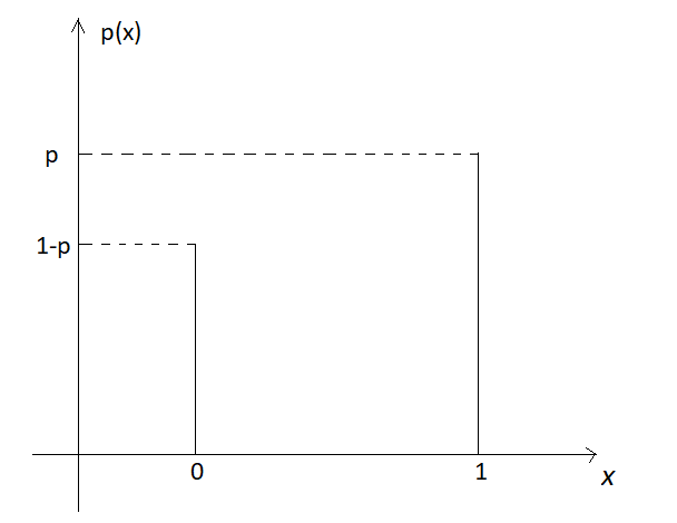
Figure 4.2: Bernoulli distribution

Example 4.19 Toss a (not necessarily fair) coin, let \[X = \begin{cases} 1 & \text{if head is obtained} \\ 0 & \text{if tail is obtained} \end{cases}\] Then \(X\) is a Bernoulli random variable.

Example 4.20 Pick a random person on a street. Let \[X = \begin{cases} 1 & \text{if the person is female} \\ 0 & \text{if the person is non-female} \end{cases}\] Then \(X\) is a Bernoulli random variable.

The expected value of \(X\) is \[\mathbb{E}(X) = \sum_{x=0}^1 xp(x) = 0 \times (1-p) + 1 \times p = p\]

Exercise 4.10 Prove that if \(X \sim \text{Bernoulli}(p)\), then \[\mathrm{var}(X) = p(1-p)\]

Notes: In this book, I only list the Bernoulli distribution as an example of discrete probability distributions. There are other popular distributions such as Binomial distribution, Geometric distribution, Poisson distribution, etc. The pmf and cdf of these distributions also possess the general properties of pmf and cdf presented in this Section.

4.4 Probability Function for Continuous Random Variables

4.4.1 Corresponding Definitions for Continuous Random Variables

In Section 4.2.3, we have discussed that for a continuous random variable \(X\), \(P(X = x) = 0\) for all possible values \(x\). Hence, we need to define the probability distribution using the probability density function (or pdf) \(f(x)\). We also need to replace the sum in the discrete case by the integral for the continuous case.

Specifically, for a continuous random variable \(X\)

• The probability density function \(f(x)\) represents the height of the density curve at the point \(x\). \(f(x) \ge 0\) for all \(x\).

• The probability of an interval \((a,b)\) is calculated as the area under the \(f(x)\) curve from \(x = a\) to \(x = b\), which is the integral \[\mathbb{P}((a,b)) = \mathbb{P}(X \in (a,b)) = \mathbb{P}(a < X < b) = \int_{a}^bf(x)dx\]

  • Because \(\mathbb{P}(X = x) = 0\), we have \[\mathbb{P}(a < X < b) = \mathbb{P}(a \le X < b) = \mathbb{P}(a < X \le b) = \mathbb{P}(a \le X \le b)\]

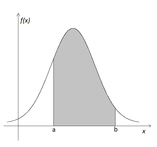
Figure 4.3: Area under the curve

• The cumulative distribution function (cdf) of \(X\) is \[F(x) = \mathbb{P}(X \le x) = \mathbb{P}(X\in(-\infty, x]) = \int_{-\infty}^x f(z)dz\]

  • The total area under the curve is \(1\), i.e., \[\mathbb{P}(\Omega) = F(+\infty) = \int_{-\infty}^{+\infty}f(x)dx = 1.\]

• The expectation of \(X\) is \[\mu_X = \mathbb{E}(X) = \int_{-\infty}^{+\infty}xf(x)dx\]

• The variance of \(X\) is \[\sigma^2_X = \mathrm{var}(X) = \mathbb{E}[(X-\mu_X)^2] = \int_{-\infty}^{+\infty}xf(x)dx\]

• The expected value of \(g(X)\) for a function \(g\) is \[\mathbb{E}[g(X)] = \int_{-\infty}^{+\infty} g(x)f(x)dx\]

It is best to explain these new concepts by an example of a continuous probability distribution.

4.4.2 Continuous Uniform Distribution

For constants \(c,d\), if \(X\) is a random variable taking on values in the interval \([c,d]\) where \(f(x)\) is the same for all \(x \in [c,d]\), then we say that \(X\) follows a Continuous uniform distribution on interval \([c,d]\). Denote \[X \sim \text{Unif}(c,d)\] The probability distribution: suppose \(f(x) = k\) for all \(c \le x \le d\) and some constant \(k\). Because \(\mathbb{P}(\Omega) = 1\), \(f(x)\) has to satisfy \[\mathbb{P}(\Omega) = \int_{-\infty}^{+\infty}f(x)dx = \int_c^d k dx = kx\Big|_{c}^d = 1 \hspace{5mm}\Rightarrow \hspace{5mm} k = \frac{1}{d-c}\] Therefore, the probability density function of \(X \sim \text{Unif}(c,d)\) is \[f(x) = \begin{cases} \frac{1}{d-c} & \text{for } c \le x \le d \\ 0 & \text{otherwise}\end{cases}\] and it can be plotted as follows.

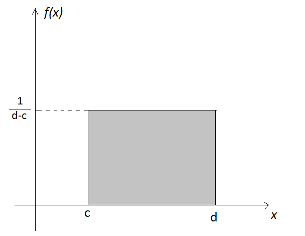
Figure 4.4: Continuous uniform distribution

The cumulative distribution of \(X\) is \[F(x) = \int_{-\infty}^{x}f(z)dz = \int_{c}^x\frac{1}{d-c}dx = \begin{cases} 0 & \text{for } x < c \\ \frac{x-c}{d-c} & \text{for } c \le x < d \\ 1 & \text{for } x \ge d \end{cases} \]

Exercise 4.11 Prove that the expected value and variance of \(X \sim \text{Unif}(c,d)\) are \[\mathbb{E}(X) = \frac{d+c}{2} \hspace{5mm} \text{and} \hspace{5mm} \mathrm{var}(X) = \frac{(d-c)^2}{12}\]

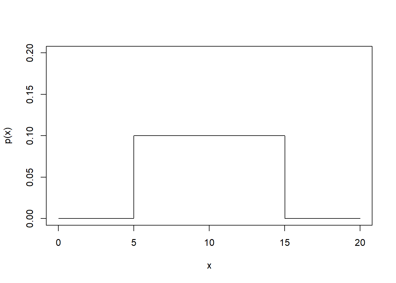
Example 4.21 Suppose the area of a room for rent for a student is a uniform random variable with values between \(5\) to \(15\) \(\mathrm{m}^2\).

Let \(X\): the the area of a student room.

1. Graph the probability distribution of \(X\).

2. On average, how big is a student room? And what is the standard deviation?

3. What is the probability that a room is less than 11.5 \(\mathrm{m}^2\)?

4. Eighty percent of the time, the area of the student room falls below what value (i.e., what is the 0.8 quantile)?

Solution:

1. See the graph below.

2. \(\mathbb{E}(X) = \frac{15+5}{2} = 10 (\mathrm{m}^2)\)

   \(\mathrm{var}(X) = \frac{(15-5)^2}{12} = 8.333\)

   \(\mathrm{sd}(X) = \sqrt{8.333} = 2.887\).

3. \(\mathbb{P}(X \le 11.5) = \frac{11.5-5}{15-5} = 0.65\)

4. \(\mathbb{P}(X \le k) = \frac{k-5}{15-5} = 0.8\), so \(k = 13\).

Exercise 4.12 The amount of time in minutes, that a person must wait for a bus is uniformly distributed between zero and \(20\) minutes.

1. Graph the probability density function. You may use R.

2. Find \(\mathbb{P}(X > 15)\).

3. Find the \(75\)th percentile.

Notes: Again, there are other examples of continuous probability distributions, for example the normal distribution, \(F\) distribution, \(t\) distribution, etc. Exceptionally, the normal distribution is a very important probability distribution in statistics. We will go over it in Chapter 5.

4.5 Comparison of Discrete and Continuous Random Variables

	Discrete RVs	Continuous RVs
Set of possible values	countable	uncountable
Probability function	Probability mass function (pmf): \(p(x) = \mathbb{P}(X = x)\)	Probability density function (pdf): \(f(x)\)
Probability of events	Sum of values in the event: \(\sum_{x \text{ of event}}p(x)\)	Integral over the interval of the event: \(\mathbb{P}(a < X < b) = \int_{a}^bf(x)dx\)
Mean	\(\mathbb{E}(X) = \sum_{\text{all }x}xp(x)\)	\(\mathbb{E}(X) = \int_{-\infty}^{\infty}xf(x)dx\)
Expectation of a function	\(\mathbb{E}(g(X)) = \sum_{\text{all }x}g(x)p(x)\)	\(\mathbb{E}(g(X)) = \int_{-\infty}^{\infty}g(x)f(x)dx\)
Examples	Bernoulli, Binomial, Geometric, Poisson distributions	Continuous uniform, Normal, \(F\)-, \(t\)-distributions

Notes: First, note that the concepts of cumulative distribution function and expectation only apply to random variables that output numeric values. For example, consider tossing a coin and two random variables \[X = \begin{cases} \text{"yes"} & \text{if a head is obtained} \\ \text{"no"} & \text{otherwise} \end{cases} \hspace{5mm} \text{and} \hspace{5mm} Y = \begin{cases} 1 & \text{if a head is obtained} \\ 0 & \text{otherwise} \end{cases}\] Then concepts of cumulative distribution function and expectations only apply to \(Y\).

Second, in this chapter, we learn about important concepts in the subject of probability: random variables, probability functions and expectations, etc. Some of them can be challenging to understand correctly, even for me. Therefore, I went at length to explain those concepts clearly with many examples. To sharpen your understanding, practice the examples, exercises and practice questions in this chapter by yourself.

---

9. You can also choose to choose other variables with different set of categories to represent “gender”. Here, we are considering the specific variable we defined in Example 4.2.↩︎

10. We will discuss about what probability density is in Section 4.4 below.↩︎

11. All possible values of \(X\) represent mutually exclusive events that make up the sample space \(\Omega\). Therefore, we can sum the probabilities of these events to get \(\mathbb{P}(\Omega)\).↩︎

12. Here, round bracket means we exclude the number, square bracket means we include the number. For example, \([1,3)\) means all the numbers from 1 to 3, including 1 but excluding 3.↩︎

13. The one we discussed in Chapter 3↩︎

14. Alternative solution: \(\mathbb{P}(X < 8) = \mathbb{P}(X \le 8) - \mathbb{P}(X = 8) = 0.75-0.25=0.5\).↩︎

15. Here, let us ignore that we use \(n-1\) instead of \(n\) for the formula of \(s^2\) because \(n\) and \(n-1\) behave very similarly when \(n\) is very large.↩︎